
T test
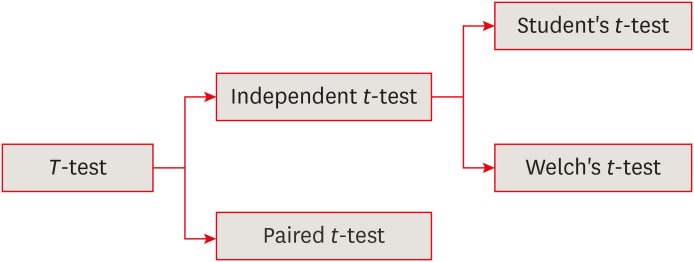
The t-test is frequently used in comparing 2 group means. The compared groups may be independent to each other such as men and women. Otherwise, compared data are correlated in a case such as comparison of blood pressure levels from the same person before and after medication . In this section we will focus on independent t-test only. There are 2 kinds of independent t-test depending on whether 2 group variances can be assumed equal or not. The t-test is based on the inference using t-distribution.
T-DISTRIBUTION
The t-distribution was invented in 1908 by William Sealy Gosset, who was working for the Guinness brewery in Dublin, Ireland. As the Guinness brewery did not permit their employee’s publishing the research results related to their work, Gosset published his findings by a pseudonym, “Student.” Therefore, the distribution he suggested was called as Student’s t-distribution. The t-distribution is a distribution similar to the standard normal distribution, z-distribution, but has lower peak and higher tail compared to it
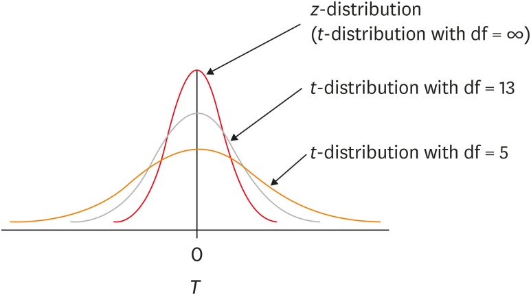
According to the sampling theory, when samples are drawn from a normal-distributed population, the distribution of sample means is expected to be a normal distribution. When we know the variance of population, σ2, we can define the distribution of sample means as a normal distribution and adopt z-distribution in statistical inference. However, in reality, we generally never know σ2, we use sample variance, s2, instead. Although the s2 is the best estimator for σ2, the degree of accuracy of s2 depends on the sample size. When the sample size is large enough (e.g., n = 300), we expect that the sample variance would be very similar to the population variance. However, when sample size is small, such as n = 10, we could guess that the accuracy of sample variance may be not that high. The t-distribution reflects this difference of uncertainty according to sample size. Therefore the shape of t-distribution changes by the degree of freedom (df), which is sample size minus one (n − 1) when one sample mean is tested.
The t-distribution appears to be a family of distribution of which shape varies according to its df . When df is smaller, the t-distribution has lower peak and higher tail compared to those with higher df. The shape of t-distribution approaches to z-distribution as df increases. When df gets large enough, e.g., n = 300, t-distribution is almost identical with z-distribution. For the inferences of means using small samples, it is necessary to apply t-distribution, while similar inference can be obtain by either t-distribution or z-distribution for a case with a large sample. For inference of 2 means, we generally use t-test based on t-distribution regardless of the sizes of sample because it is always safe, not only for a test with small df but also for that with large df.
INDEPENDENT SAMPLES T-TEST
To adopt z– or t-distribution for inference using small samples, a basic assumption is that the distribution of population is not significantly different from normal distribution. As seen in Appendix 1, the normality assumption needs to be tested in advance. If normality assumption cannot be met and we have a small sample (n < 25), then we are not permitted to use ‘parametric’ t-test. Instead, a non-parametric analysis such as Mann-Whitney U test should be selected.
For comparison of 2 independent group means, we can use a z-statistic to test the hypothesis of equal population means only if we know the population variances of 2 groups, 𝜎21 and 𝜎22, as follows;
| 𝑍 = −𝑋1 − −𝑋2√𝜎21𝑛1 + 𝜎22𝑛2 | (Eq. 1) |
where X̄1 and X̄2, 𝜎21 and 𝜎22, and n1 and n2 are sample means, population variances, and the sizes of 2 groups.
Again, as we never know the population variances, we need to use sample variances as their estimates. There are 2 methods whether 2 population variances could be assumed equal or not. Under assumption of equal variances, the t-test devised by Gosset in 1908, Student’s t-test, can be applied. The other version is Welch’s t-test introduced in 1947, for the cases where the assumption of equal variances cannot be accepted because quite a big difference is observed between 2 sample variances
1. Student's t-test
In Student’s t-test, the population variances are assumed equal. Therefore, we need only one common variance estimate for 2 groups. The common variance estimate is calculated as a pooled variance, a weighted average of 2 sample variances as follows;
| 𝑠2𝑝 = (𝑛1 − 1)(𝑛1 − 1)+(𝑛2 − 1)𝑠21 + (𝑛2 − 1)(𝑛1 − 1)+(𝑛2 − 1)𝑠22 | (Eq. 2) |
where 𝑠21 and 𝑠22 are sample variances.
The resulting t-test statistic is a form that both the population variances, 𝜎21 and 𝜎21, are exchanged with a common variance estimate, 𝑠2p. The df is given as n1 + n2 − 2 for the t-test statistic.
| 𝑡 = −𝑋1 − −𝑋2√𝑠2𝑝𝑛1 + 𝑠2𝑝𝑛2 = −𝑋1 − −𝑋2𝑠𝑝√1𝑛1 + 1𝑛2~𝑡(𝑛1 + 𝑛2 − 2) | (Eq. 3) |
In Appendix 1, ‘(E-1) Leven’s test for equality of variances’ shows that the null hypothesis of equal variances was accepted by the high p value, 0.334 (under heading of Sig.). In ‘(E-2) t-test for equality of means t-values’, the upper line shows the result of Student’s t-test. The t-value and df are shown −3.357 and 18. We can get the same figures using the formulas Eq. 2 and Eq. 3, and descriptive statistics.
| Group | No. | Mean | Standard deviation | p value |
|---|---|---|---|---|
| 1 | 10 | 10.28 | 0.5978 | 0.004 |
| 2 | 10 | 11.08 | 0.4590 |
| 𝑠2𝑝 = (10 − 1) × 0.59782 + (10 − 1) × 0.45902(10 − 1) + (10 − 1) = 5.112418 = 0.2840 = (0.5329)2 |
| 𝑡 = −𝑋1 − −𝑋2𝑠𝑝√1𝑛1 + 1𝑛2 = 10.28 − 11.080.5329√19 + 19 = −0.800.2512 = −3.18 |
| df = n1 + n2 − 2 = 10 + 10 − 2 = 18 |
The result of calculation is a little different from that by SPSS (IBM Corp., Armonk, NY, USA) of Appendix 1, maybe because of rounding errors.
2. Welch's t-test
Actually there are a lot of cases where the equal variance cannot be assumed. Even if it is unlikely to assume equal variances, we still compare 2 independent group means by performing the Welch’s t-test. Welch’s t-test is more reliable when the 2 samples have unequal variances and/or unequal sample sizes. We need to maintain the assumption of normality.
Because the population variances are not equal, we have to estimate them separately by 2 sample variances, 𝑠21 and 𝑠22. As the result, the form of t-test statistic is given as follows;
| 𝑡 = −𝑋1 − −𝑋2√𝑠21𝑛1 + 𝑠22𝑛2~𝑡𝜈 | (Eq. 4) |
where ν is Satterthwaite degrees of freedom.
| 𝜈 = 𝑠21𝑛1 + 𝑠22𝑛2(𝑠21𝑛1)2/(𝑛1 − 1) + (𝑠22𝑛2)2/(𝑛2 − 1) | (Eq. 5) |
In Appendix 1, ‘(E-1) Leven’s test for equality of variances’ shows an equal variance can be successfully assumed (p = 0.334). Therefore, the Welch’s t-test is inappropriate for this data. Only for the purpose of exercise, we can try to interpret the results of Welch’s t-test shown in the lower line in ‘(E-2) t-test for equality of means t-values’. The t-value and df are shown as −3.357 and 16.875.
| 𝑡 = −𝑋1 − −𝑋2√𝑠21𝑛1 + 𝑠22𝑛2 = 10.28 − 11.08√0.5978210 + 0.4590210 = −0.800.2383 = −3.357 |
| 𝜐 = (𝑠21𝑛1 + 𝑠22𝑛2)2(𝑠21𝑛1)2/(𝑛1 − 1) + (𝑠22𝑛2)2/(𝑛2 − 1) = (0.5978210 + 0.4590210)2(0.5978210)210−1 + (0.4590210)210−1 = 0.0567920.0001419 + 0.0000493 = .0032250.0001912 ≅ 16.87 |
We’ve confirmed nearly same results by calculation using the formula and by SPSS software.
The t-test is one of frequently used analysis methods for comparing 2 group means. However, sometimes we forget the underlying assumptions such as normality assumption or miss the meaning of equal variance assumption. Especially when we have a small sample, we need to check normality assumption first and make a decision between the parametric t-test and the nonparametric Mann-Whitney U test. Also, we need to assess the assumption of equal variances and select either Student’s t-test or Welch’s t-test
Steps to apply independent T test
Applying an independent samples t-test involves a series of steps, from setting up your hypotheses to interpreting the results. Here’s a breakdown of the process:
1. Define Your Hypotheses:
- Null Hypothesis (H0): There is no significant difference between the means of the two groups. (μ1 = μ2)
- Alternative Hypothesis (H1): There is a significant difference between the means of the two groups. (μ1 ≠ μ2) (This is a two-tailed test. You can also have one-tailed tests if you have a directional hypothesis.)
2. Check the Assumptions:
- Independence: The observations in each group must be independent of each other.
- Normality: The distribution of the dependent variable should be approximately normal within each group. This can be checked using histograms, Q-Q plots, or statistical tests like the Shapiro-Wilk test.
- Homogeneity of Variance: The variances of the two groups should be approximately equal. Levene’s test is commonly used to assess this.
3. Collect Your Data:
- Ensure you have two distinct, independent groups and a continuous dependent variable.
4. Perform the t-test:
- You can perform the t-test using statistical software such as:
- SPSS: Navigate to Analyze > Compare Means > Independent-Samples T Test.
- R: Use the
t.test()function. - Python (SciPy): Use the
scipy.stats.ttest_ind()function. - Other Statistical Software: Most statistical software packages provide a function for performing independent t-tests.
- When running the test, the software will calculate:
- The t-statistic.
- The degrees of freedom (df).
- The p-value.
- Also, the software will output the means and standard deviations of each of the two groups.
- Levene’s test results. This is very important to determine if equal variances were assumed, or not.
Advantages of T test
The T-test is a statistical method used to determine whether there is a significant difference between the means of two groups. It is commonly used when dealing with small sample sizes and when the population standard deviation is unknown. Here are some advantages of using a T-test:
1. Simple and Easy to Use
- The T-test is straightforward to apply, making it ideal for researchers, students, and professionals who need to compare means.
2. Suitable for Small Sample Sizes
- Unlike the Z-test, which requires large samples (usually n>30n > 30n>30), the T-test is effective even with small samples (n<30n < 30n<30).
3. Works with Unknown Population Variance
- Unlike some other statistical tests, the T-test does not require the population standard deviation to be known, making it more practical in real-world scenarios.
4. Different Variants for Different Scenarios
- There are different types of T-tests suited for various types of data:
- One-sample T-test: Compares a sample mean to a known population mean.
- Independent (two-sample) T-test: Compares the means of two independent groups.
- Paired (dependent) T-test: Compares the means of the same group before and after an intervention.
5. Helps in Hypothesis Testing
- It allows researchers to test hypotheses about differences between means and determine statistical significance.
For more query contact:Grow@simbi.in
Frequently
Asked Questions
There are three main types of T-tests:
- One-sample T-test: Compares the mean of a single group to a known value or population mean.
- Independent (two-sample) T-test: Compares the means of two different (independent) groups.
- Paired (dependent) T-test: Compares means from the same group at different times (e.g., before and after treatment).
Use a T-test when:
- You want to compare the means of two groups.
- The sample size is small (n<30n < 30n<30).
- The data is approximately normally distributed.
- The population standard deviation is unknown
A T-test requires:
- Normality – The data should be approximately normally distributed (especially for small samples).
- Independence – Observations should be independent of each other.
- Equal variance (for independent T-test only) – The two groups should have roughly equal variances (can be relaxed using Welch’s T-test).
The general formula for a T-test is:
t=Observed difference in meansStandard error of the differencet = \frac{\text{Observed difference in means}}{\text{Standard error of the difference}}t=Standard error of the differenceObserved difference in means
For an independent two-sample T-test:
t=X1ˉ−X2ˉs12n1+s22n2t = \frac{\bar{X_1} - \bar{X_2}}{\sqrt{\frac{s_1^2}{n_1} + \frac{s_2^2}{n_2}}}t=n1s12+n2s22X1ˉ−X2ˉ
Where:
- X1ˉ,X2ˉ\bar{X_1}, \bar{X_2}X1ˉ,X2ˉ = Sample means
- s12,s22s_1^2, s_2^2s12,s22 = Sample variances
- n1,n2n_1, n_2n1,n2 = Sample sizes
For a paired T-test, the formula is:
t=dˉsd/nt = \frac{\bar{d}}{s_d / \sqrt{n}}t=sd/ndˉ
Where:
- dˉ\bar{d}dˉ = Mean of the differences
- sds_dsd = Standard deviation of the differences
- nnn = Number of paired observations
The null hypothesis states that there is no significant difference between the means of the two groups.
For example:
- One-sample T-test: H0:μ=μ0H_0: \mu = \mu_0H0:μ=μ0 (The sample mean is equal to the population mean)
- Independent T-test: H0:μ1=μ2H_0: \mu_1 = \mu_2H0:μ1=μ2 (The means of two independent groups are equal)
- Paired T-test: H0:μd=0H_0: \mu_d = 0H0:μd=0 (The mean difference between paired samples is zero)
The alternative hypothesis states that there is a significant difference between the means.
For example:
- Two-tailed test: HA:μ1≠μ2H_A: \mu_1 \neq \mu_2HA:μ1=μ2 (The means are different)
- One-tailed test: HA:μ1>μ2H_A: \mu_1 > \mu_2HA:μ1>μ2 or HA:μ1<μ2H_A: \mu_1 < \mu_2HA:μ1<μ2 (One mean is greater/lesser than the other)