
Meta-Analysis in R-Software: A Practical Guide with Case Studies on Continuous and Dichotomous Data

Part A: Meta Analysis for Continuous Data:
Case Study 1:
Research Question
Does physical activity improve self-esteem in adolescents compared to no intervention?
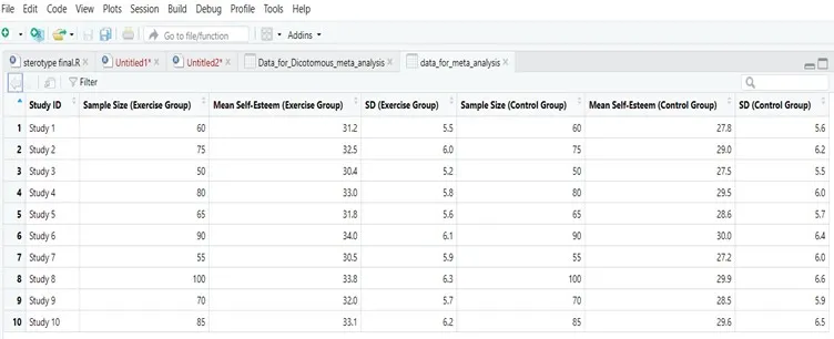
Data:
| Study ID | Sample Size (Exercise Group) | Mean Self-Esteem (Exercise Group) | SD (Exercise Group) | Sample Size (Control Group) | Mean Self-Esteem (Control Group) | SD (Control Group) |
| Study 1 | 60 | 31.2 | 5.5 | 60 | 27.8 | 5.6 |
| Study 2 | 75 | 32.5 | 6 | 75 | 29 | 6.2 |
| Study 3 | 50 | 30.4 | 5.2 | 50 | 27.5 | 5.5 |
| Study 4 | 80 | 33 | 5.8 | 80 | 29.5 | 6 |
| Study 5 | 65 | 31.8 | 5.6 | 65 | 28.6 | 5.7 |
| Study 6 | 90 | 34 | 6.1 | 90 | 30 | 6.4 |
| Study 7 | 55 | 30.5 | 5.9 | 55 | 27.2 | 6 |
| Study 8 | 100 | 33.8 | 6.3 | 100 | 29.9 | 6.6 |
| Study 9 | 70 | 32 | 5.7 | 70 | 28.5 | 5.9 |
| Study 10 | 85 | 33.1 | 6.2 | 85 | 29.6 | 6.5 |
Data Description:
The dataset includes summary statistics from 10 studies comparing self-esteem scores between exercise and control groups, each providing sample size, mean, and standard deviation.
Saving this Data in Excel for Meta-Analysis in R Software
Step by Step Meta Analysis for Continuous data in R Software:
Step 1: Load Packages and Data in R Software
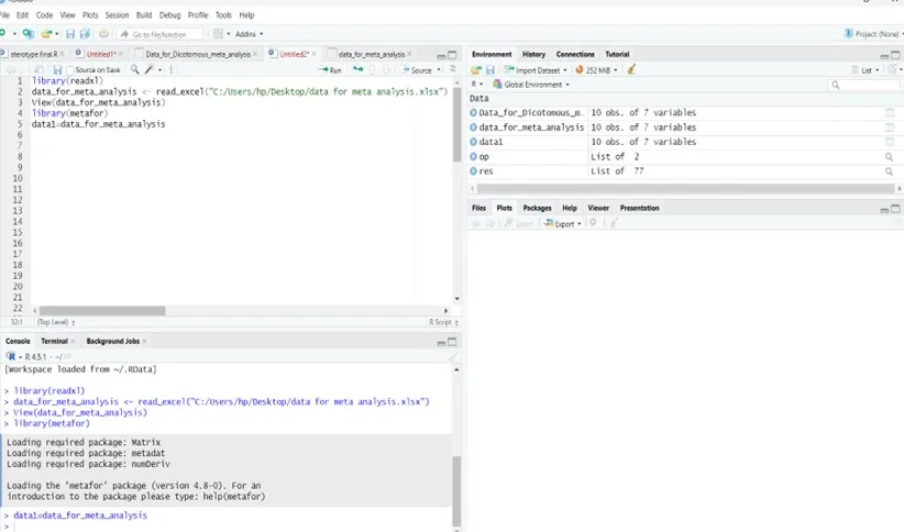
Data View in R Software:
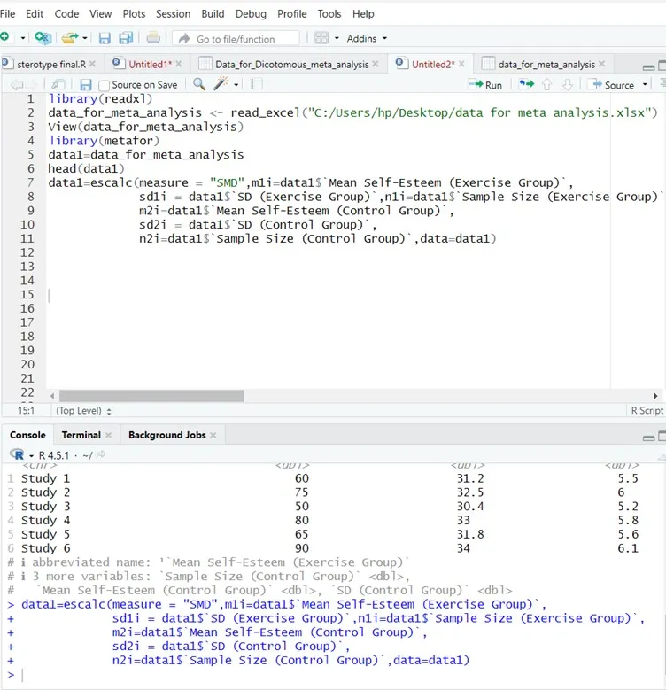
Step 2: Calculate Effect Sizes (Method= Standardized Mean Difference (SMD))
Step 3: Run Random-Effects Meta-Analysis
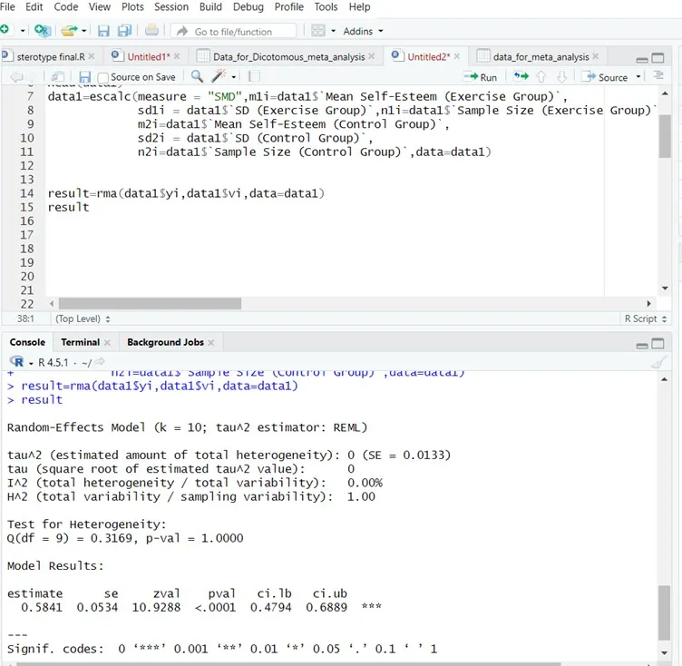
R Software Output Summary:
| Random-Effects Model (k = 10; tau^2 estimator: REML) |
| tau^2 (estimated amount of total heterogeneity): 0 (SE = 0.0133) |
| tau (square root of estimated tau^2 value): 0 |
| I^2 (total heterogeneity / total variability): 0.00% |
| H^2 (total variability / sampling variability): 1.00 |
| Test for Heterogeneity: |
| Q(df = 9) = 0.3169, p-val = 1.0000 |
| Model Results: |
| estimate se zval pval ci.lb ci.ub |
| 0.5841 0.0534 10.9288 <.0001 0.4794 0.6889 *** |
| — |
| Signif. codes: 0 ‘***’ 0.001 ‘**’ 0.01 ‘*’ 0.05 ‘.’ 0.1 ‘ ’ 1 |
Interpretation:
The pooled Effect is 0.58 and statistically significant (p < 0.0001), indicating higher self-esteem in the exercise group. No heterogeneity is observed among the studies (I² = 0%, τ² = 0, Q-test p = 1.00). This suggests that the effect is consistent across all 10 studies.
Step 4: Forest Plot
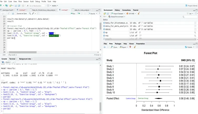
Forest Plot:
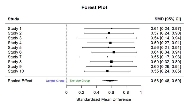
Interpretation:
All studies report positive standardized mean differences (SMDs) ranging from 0.54 to 0.64, indicating a consistent moderate effect of physical activity on adolescent self-esteem. Since none of the 95% confidence intervals include zero, each individual effect is statistically significant. The overall pooled SMD is 0.58 [95% CI: 0.48, 0.69], confirming a moderate and reliable positive impact of physical activity on self-esteem.
Step 5: Funnel Plot and Egger’s Test (Publication Bias)
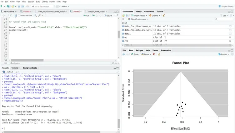
Funnel Plot:
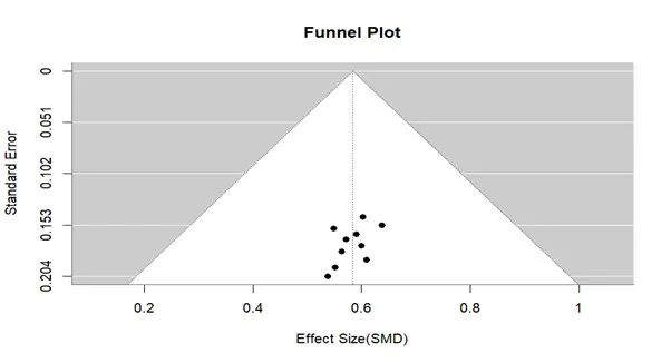
Interpretation:
The Funnel Plot Seems Symmetrical Suggest No Publication Bias
Eggers Test Hypothesis:
Null Hypothesis (H₀):
There is no funnel plot asymmetry — the effect sizes are not related to their standard errors.
This implies no publication bias or small-study effects.
Alternative Hypothesis (H₁):
There is funnel plot asymmetry — the effect sizes are related to their standard errors.
This suggests potential publication bias or small-study effects.
R Software Output Eggers Test:
Regression Test for Funnel Plot Asymmetry
Model: mixed-effects meta-regression model
Predictor: standard error
Test for Funnel Plot Asymmetry: z = -0.2845, p = 0.7761
Limit Estimate (as sei -> 0): b = 0.7305 (CI: -0.2832, 1.7442)
Interpretation:
Since the p-value is 0.7761 (greater than 0.05), we fail to reject the null hypothesis.
This means there is no statistical evidence of funnel plot asymmetry, and hence no indication of publication bias in the meta-analysis.
Part B: Meta Analysis for Dichotomous Data:
Case Study 2:
Research Question:
Does Drug A reduce the risk of infection compared to Placebo?
Data
| Study ID | Drug A Events | Drug A No Events | Drug A Total | Placebo Events | Placebo No Events | Placebo Total |
| Study 1 | 12 | 90 | 102 | 25 | 79 | 104 |
| Study 2 | 18 | 84 | 102 | 30 | 73 | 103 |
| Study 3 | 10 | 90 | 100 | 20 | 80 | 100 |
| Study 4 | 8 | 94 | 102 | 16 | 86 | 102 |
| Study 5 | 20 | 82 | 102 | 35 | 70 | 105 |
| Study 6 | 15 | 85 | 100 | 28 | 78 | 106 |
| Study 7 | 17 | 85 | 102 | 33 | 68 | 101 |
| Study 8 | 13 | 89 | 102 | 27 | 80 | 107 |
| Study 9 | 19 | 70 | 89 | 31 | 70 | 101 |
| Study 10 | 14 | 86 | 100 | 26 | 80 | 106 |
Data Description:
The dataset includes results from 10 studies comparing infection rates between patients receiving Drug A and those receiving a placebo. Each study reports the number of infection events and non-events in both groups as well as Total enabling the calculation of risk Differences.
Saving this Data in Excel for Meta-Analysis in R Software
Step by Step Meta Analysis for Dichotomous Data in R Software:
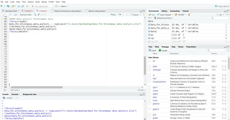
Data View in R Software:

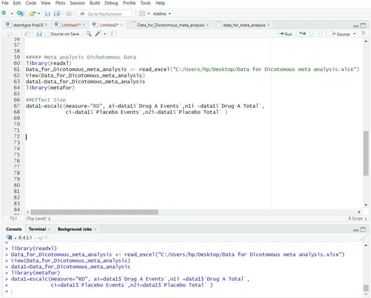
Step 2: Calculate Effect Sizes (Method= Risk Difference (RD))
Step 3: Run Random-Effects Meta-Analysis
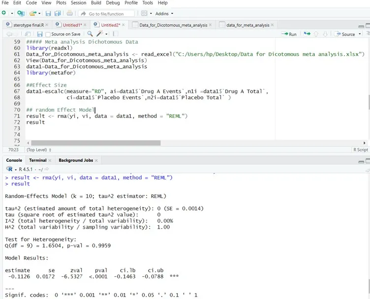
R Software Output Summary:
| Random-Effects Model (k = 10; tau^2 estimator: REML) |
| tau^2 (estimated amount of total heterogeneity): 0 (SE = 0.0014) |
| tau (square root of estimated tau^2 value): 0 |
| I^2 (total heterogeneity / total variability): 0.00% |
| H^2 (total variability / sampling variability): 1.00 |
| Test for Heterogeneity: |
| Q(df = 9) = 1.6504, p-val = 0.9959 |
| Model Results: |
| estimate se zval pval ci.lb ci.ub |
| -0.1126 0.0172 -6.5327 <.0001 -0.1463 -0.0788 *** |
| — |
| Signif. codes: 0 ‘***’ 0.001 ‘**’ 0.01 ‘*’ 0.05 ‘.’ 0.1 ‘ ’ 1 |
Interpretation:
The pooled risk difference is –0.11 (p < 0.0001), indicating that Drug A reduces the infection risk by 11 percentage points compared to placebo. The 95% confidence interval [–0.15, –0.08] confirms that this reduction is statistically significant. With I² = 0%, there is no heterogeneity, meaning the treatment effect is consistent across all studies.
Step 4: Forest Plot
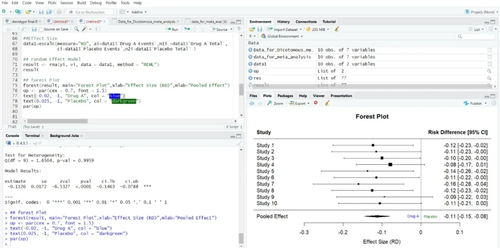
Forest Plot:
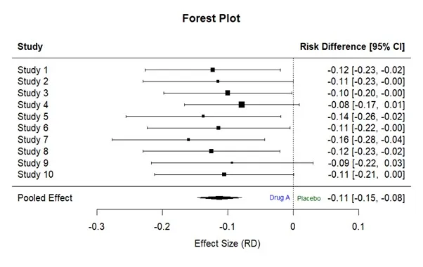
Interpretation:
All studies report negative risk differences (RDs) ranging from –0.08 to –0.16, indicating a consistent reduction in infection risk with Drug A compared to placebo. The overall pooled risk difference is –0.11 [95% CI: –0.15, –0.08], confirming a moderate and reliable absolute reduction in infection risk due to Drug A.
Step 5: Funnel Plot and Egger’s Test (Publication Bias)
Funnel Plot:
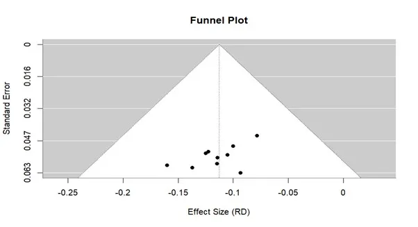
Interpretation:
The Funnel Plot Seems Symmetrical Suggest No Publication Bias
Eggers Test Hypothesis:
Null Hypothesis (H₀):
There is no funnel plot asymmetry — the effect sizes are not related to their standard errors.
This implies no publication bias or small-study effects.
Alternative Hypothesis (H₁):
There is funnel plot asymmetry — the effect sizes are related to their standard errors.
This suggests potential publication bias or small-study effects.
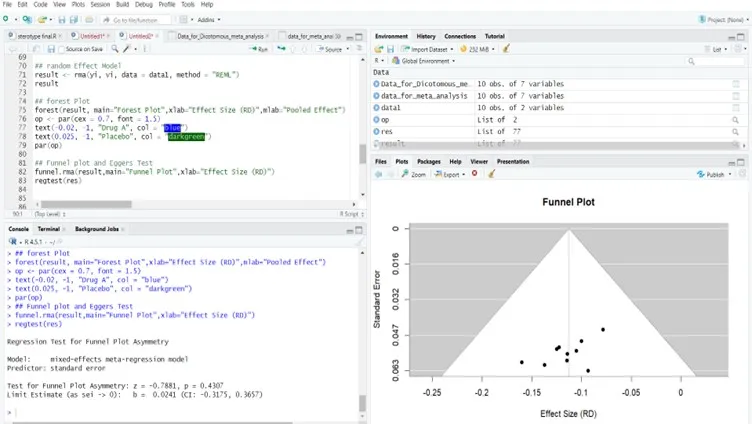
R Software Output Eggers Test:
Regression Test for Funnel Plot Asymmetry
Model: mixed-effects meta-regression model
Predictor: standard error
Test for Funnel Plot Asymmetry: z = -0.7881, p = 0.4307
Limit Estimate (as sei -> 0): b = 0.0241 (CI: -0.3175, 0.3657)
Interpretation:
Since the p-value is 0.4307 (greater than 0.05), we fail to reject the null hypothesis.
This means there is no statistical evidence of funnel plot asymmetry, and hence no indication of publication bias in the meta-analysis.