
Introduction:
Central tendency is an important idea in statistics. It helps us understand a group of numbers by finding one value that best represents the whole group. In this blog, we’ll look at the basic types of central tendency—mean, median, mode, and standard deviation. We’ll also talk about the good and bad sides of each and how they are used in real life.
Example 1: Suppose, one of your relative ask you about your exam result. If you explain the marks of every subjects separately, he/she will become boring and would not able understand your performance.
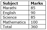
What will you do? You will answer 90%.
This is the central value of your marks score in different subjects
Example 2:
Suppose, you are a class teacher. Marks
score by five students in a test is given below. Will you able to compare the
performance of these students by comparing the marks score in different
subjects separately.
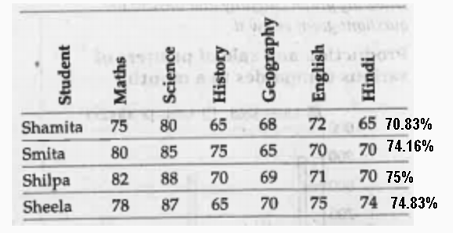
What will you do? You will compare by their percentage.
This is the central value of marks score by the five students in the test.
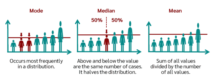
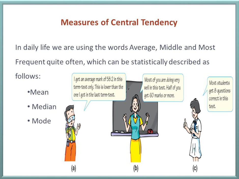
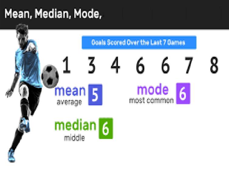
Measures of central tendency
Mean:
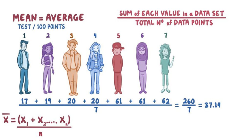
Definition: The mean is the average of a set of numbers. It is calculated by summing all the values in the dataset and dividing the sum by the number of values
For Ungrouped Data:
If the variable x assumes n values x1, x2 … xn, then the mean is given by
x̅ = (x₁ + x₂ + x₃ + ... + xₙ) / n
Example: Suppose marks scored by five students in a test is 66, 72, 85, 52, and 75.
x̅
= (66+72+85+52+75)/5
=350/5
=70
Mean: For Grouped data
x̅= (∑fx)/n
x = the mid-point of individual class,
f = the frequency of individual class
N = the sum of the frequencies or total frequencies in a sample.
For example
(∑fx)/n =1320/50=38
| Marks | No. of Students (f) | x | Fx |
| 0-10 | 6 | 5 | 30 |
| 10-20 | 8 | 15 | 120 |
| 20-30 | 17 | 25 | 425 |
| 30-40 | 11 | 35 | 385 |
| 40-50 | 8 | 45 | 360 |
| N=50 | 1,320 |
Merits:
1. Easy to understand and calculate.
2. It is clearly defined.
3. Uses all values in the data
4. Sensitive to small changes in values.
5. Common in advance statistics.
6. Works with both discrete and continuous data.
7. Useful for comparison.
Demerits:
- You can’t find it just by looking or from a graph.
- It cannot be in the study of qualitative phenomena not capable of numerical measurement i.e., Intelligence, beauty, honesty etc.,
- It can ignore any single item only at the risk of losing its accuracy.
- It changes a lot if there are very big or very small numbers in the data.
- It cannot be calculated for open-end classes.
- It can give you the wrong idea if you don’t the full details of data.
Some more examples:
1) Consider the following dataset representing the salaries of employees in a small company: {30000, 35000, 40000, 45000, 50000}
Mean= (30,000+35,000+40,000+45,000+50,000)/5
= 200,000/5
= 40,000
Now, let’s introduce an extreme value, such as the CEO’s salary, which is significantly higher: {30000, 35000, 40000, 45000, 500000}
Recalculating the mean = (30,000+35,000+40,000+45,000+500,000)/5</p> <p> =[latex]6,50,000/5
= 1,30,000
2) The Per capita Income of India is Rs. 1,72,000 and the BPL income limit in India is Rs. 27,000.
India should not have any PBL population, But India has more than 145.71 million or 10.2% of the total population.
Mean interpretation of SPSS data table :
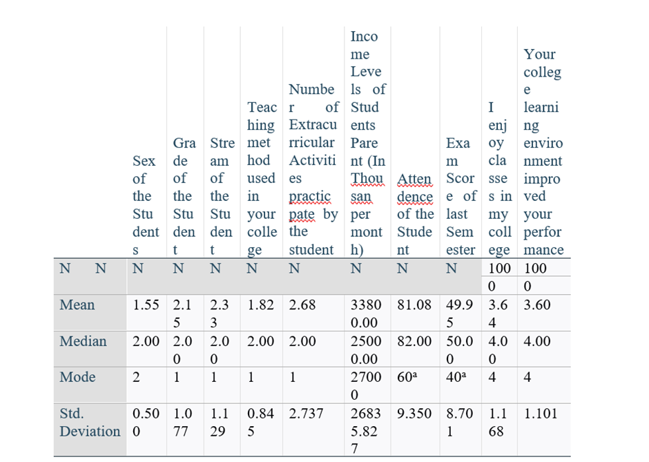
Interpretation of Mean:
Variable name: 1) Number of Extracurricular Activities participated by the student
The mean of 2.68 indicates that, on average, each student participates in approximately 2.68 extracurricular activities.
This mean suggests a moderate level of participation in extracurricular activities among the students surveyed. While not exceptionally high, it indicates that students are somewhat involved in activities beyond their regular academic curriculum.
Variable name: 2) Income Levels of Students Parent (In Thousand per month)
The mean income of 33,800 rupees per month suggests that, on average, the parents of these 100 students earn approximately 33,800 rupees per month.
The mean income level of 33,800 rupees per month provides valuable insight into the socioeconomic context of the student population, informing decision-making processes aimed at promoting equity, access, and inclusivity in education.
- Both variables value calculated is scale or pure numeric. Therefore mean or arithmetic mean or average is used in statistical analysis.
Median
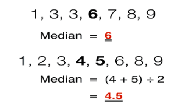
Definition: The median is the middle value in a sorted list of numbers. If there is an even number of values, it is the average of the two middle values.
The median is the middle most item that divides the group into two equal parts, one part comprising all values greater, and the other, all values less than that item.
Suppose median salary of a company is Rs. 40,000. This measure of central tendency means that one one-half of all employee earn more than 40,000, and one-half earn less than 40,000.

Ungrouped or Raw data
Arrange the given values in ascending order. If the number of values is odd,
the median is the middle value. If the number of values are even, median is the
mean of middle two values.
When n is odd, Median =
Md = ((n+1)/2)^th value
When n is even, Median = Average of (n/2)^th and(n/2+1)^th value
Some examples:
1) The number of rooms in 7 hotels in Delhi is 713, 300, 618, 595, 311, 401, and 292. Find the median.
Here n = 7, First arrange it in ascending order:292, 300, 311, 401, 595, 618, 713
Median = ((n+1)/2)^th value=((7+1)/2)^th value=4^th value = 401
2) The number of floods that have occurred in India over an 8-year period follows. Find the median. 684, 764, 656,702, 856, 1133, 1132, 130
Here n = 8, First arrange it in ascending order: 656, 684, 702, 764, 856, 1132, 1133, 1303
Median =Average of (n/2)^th and(n/2+1)^th value
= Average of (8/2)^th and(8/2+1)^th value
= Average of 4^th and〖 5〗^th value
= (764+856)/2
= 810
Grouped data
In a grouped distribution, values are associated with frequencies. Grouping can be
in the form of a discrete frequency distribution or a continuous frequency
distribution. Whatever may be the type of distribution, cumulative frequencies
have to be calculated to know the total number of items.
Cumulative frequency (cf)
Cumulative frequency of each class is the sum of the frequency of the class and the
frequencies of the pervious classes, i.e. adding the frequencies successively,
so that the last cumulative frequency gives the total number of items.
Discrete Series
Step1: Find cumulative frequencies.
Step2: Find (n/2+1)
Step3: See in the cumulative frequencies the value just greater than (n/2+1)
Step4: Then the corresponding value of x is median
The following data pertaining to the number of customers per day in
beauty salon in Delhi. Find the median number of customers.
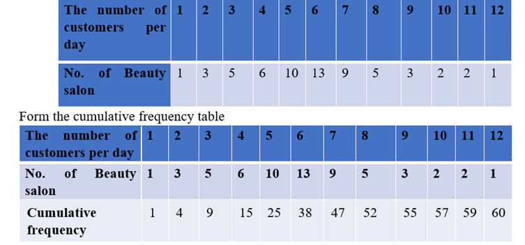
Median = size of ((n+1)/2)^th item
Here the number of observations is even.
Therefore median =average of (n/2)^th item and(n/2+1)^th item.
= (30th item +31st item) / 2 = (6+6)/2
= 6
Continuous Series
The steps given below are followed for the calculation of median in continuous series.
Step1: Find cumulative frequencies. Step2: Find (n/2) Step3: See in the cumulative frequency the value first greater than (n/2), Then the corresponding class interval is called the Median class. Then apply the formula
Median = l+(n/2-m)/f xc
where l = Lower limit of the median class,
f =frequency in the median class.
m = cumulative frequency preceding the median class,
c = width of the class
n=Total frequency
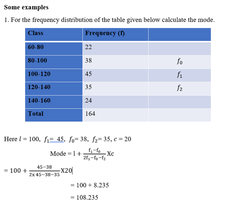
For the frequency distribution given in table below, calculate the median.
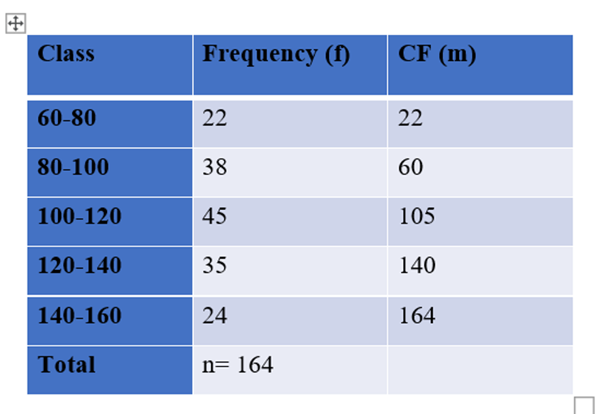
The cumulative frequency just greater than 82 is 105. Therefore, the median class is 100-120. Its lower limit is 100.
Here l = 100,
n=164 ,
f = 45 ,
c = 20,
m =60
Median = l+(N/2-C.F)*(h/f)
= 100+(164/2-60)/45 x20
= 109.78
Example: Spss data to analys Median for two ordinal Variables
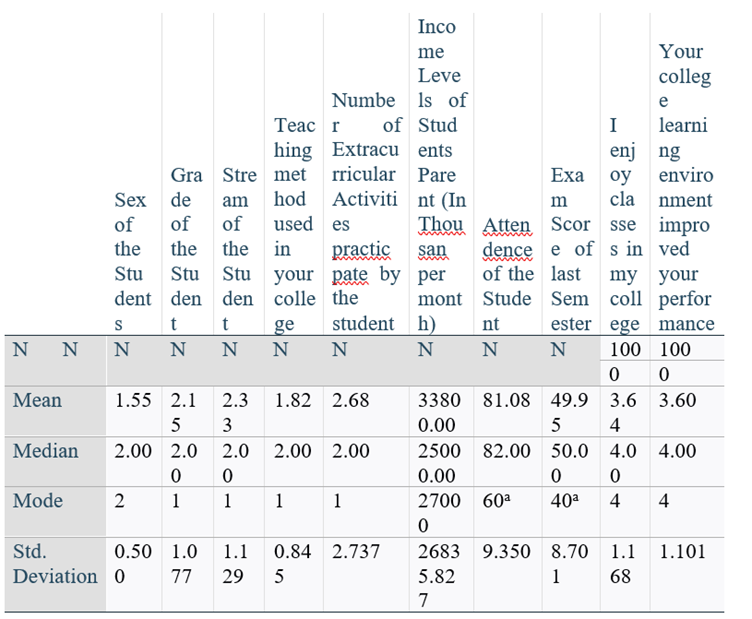
Interpretation of median:
Variable name:1) Grade of the Student
The median represents the middle value of the dataset when all grades are arranged in ascending order. In this case, with 100 students, the median indicates that approximately 50 students have grades lower than 2.00, and approximately 50 students have grades higher than 2.00.
Variable name:2) the variable "Your college learning environment improved your performance" is a subjective measure likely to be recorded on a scale (e.g., strongly agree, agree, neutral, disagree, strongly disagree), let's assume it's on a scale from 1 to 5:
This indicates that a significant portion of the student population perceives a positive impact of the college learning environment on their performance.
Both of the variables are ordinal in nature. Therefore median is used for statistical analysis.
Merits:
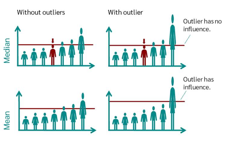
1. Not influenced by extreme values or outliers.
2. Suitable for skewed distributions.
3. Provides a better representation of the central value when the dataset is not symmetric.
4. Applicable to ordinal and interval data.
5. Robust measure of central tendency.
Demerits:
1. Tedious to compute for large datasets.
2. Ignores most of the information in the dataset.
3. Limited in its ability to reflect the variability of data.
4. Requires data to be ordered.
5. May not be unique if the dataset contains repeated values.
Some Examples
1) Consider the following dataset representing the salaries of employees in a small company: {30000, 35000, 40000, 45000, 50000} Median = 40,000
Now, let's introduce an extreme value, such as the CEO's salary, which is significantly higher: {30000, 35000, 40000, 45000, 500000} New Median = 40,000
Mode
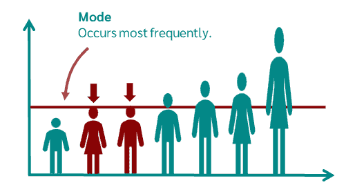
Definition: The mode is the value that appears most frequently in a dataset.
The mode refers to that value in a distribution, which occur most frequently. It is an actual value, which has the highest concentration of items in and around it. It shows the center of concentration of the frequency in around a given value. Therefore, where the purpose is to know the point of the highest concentration it is preferred.
Ungrouped or Raw Data
For ungrouped data or a series of individual observations, mode is often found by mere inspection.
Find the mode for the following data: 2, 7, 10, 15, 10, 17, 8, 10, 2 ∴Mode = 10
In some cases, the mode may be absent or there may be more than one mode.
(1) 12, 10, 15, 24, 30 (no mode)
(2) 7, 10, 15, 12, 7, 14, 24, 10, 7, 20, 10
Here, the modal values are 7 and 10 as both occur 3 times each
Continuous distribution
Locate the highest frequency the class corresponding to that frequency is called the modal class.
Then apply the formula.
Mode = l+(f_1-f_0)/(〖2f〗_1-f_0-f_2 ) xc
Where l = lower limit of the model class
f_0= the frequency of the class preceding the model class
f_1= the frequency of the model class
f_2= the frequency of the class succeeding the model class
and c = class interval
Merits:
1. Simple to understand and calculate.
2. Applicable to nominal, ordinal, and interval data.
3. Not affected by extreme values.
4. Suitable for non-parametric data analysis.
5. Useful for identifying the most common observation in a dataset.
Demerits of Mode (in Simple Words):
- May not exist if no value is repeated in the data.
- Can be confusing if more than one value appears most often (not unique).
- Doesn't show size or value differences — only tells which value occurs most.
- Small changes in data don’t affect the mode.
- Not useful for continuous data unless you group the data into categories first.
SPSS analysis for calculating mode:
Interpretation of Mode:
Variable 1 - Grade of the Student:
If the mode for the variable "Stream of the Students" is 1, it means most students are in Stream 1.
In other words, Stream 1 is the most common or popular stream among all the students in the data.
Variable 2: (e.g., Student Category or Stream)
- Mode is best used for categorical data, like nominal (e.g., stream, category) or ordinal (e.g., grade levels).
- That’s why, for variables like grade or stream, using mode helps us understand which group is chosen most often.
Summarization:
Real-world Applications with Examples
A. Finance
Example: Average Returns
1. Mean: Calculating the mean return on investment provides a measure of the average performance.
2. Median: In a scenario where extreme values can skew the mean, the median return might offer a more representative value.
B. Healthcare
Example: Patient Data Analysis
1. Mean and Median: Analyzing patient data, such as hospital stay durations, can involve both the mean and median to understand the central tendencies and potential outliers.
2. Mode: Identifying the mode in healthcare data could reveal the most frequently occurring conditions.
C. Retail
Example: Sales Data
1. Mode: In retail sales, identifying the mode of popular products can guide inventory management.
2. Mean and Median: Calculating the mean and median of sales amounts can help in understanding the central tendency of sales data.
.
A. Outliers
Example: Income Distribution
1. In a group of people’s incomes, a few who earn a lot more than others can make the average (mean) look higher than what most people actually earn. The median is not affected as much by these high incomes, so it can give a better idea of what a typical person earns.
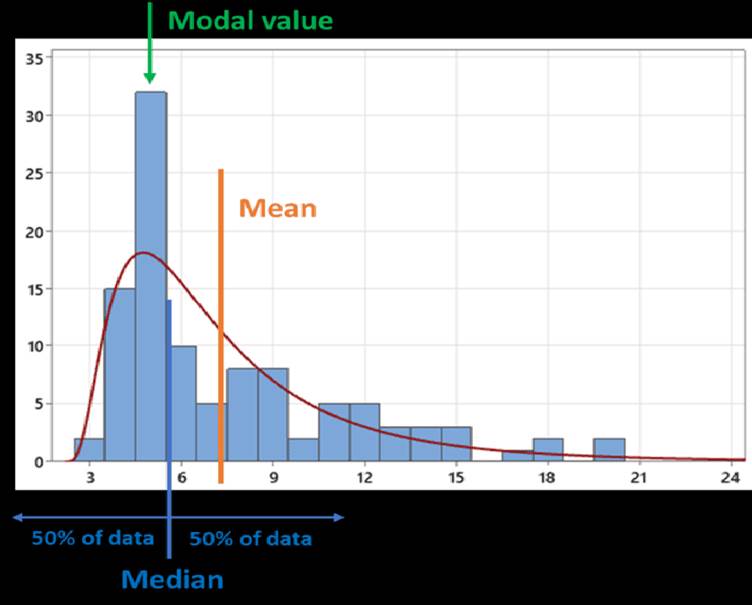
B. Skewness
Example: Exam Scores
1. In a neighborhood, most people earn around Rs. 300000 a month, but a few very rich people earn Rs. 5 Lakhs or more. Because of these high incomes, the average income looks much higher than what most people actually earn. In this case the mean is higher than the median, showing positively skewed distribution.
In real-world applications, the choice of a measure of central tendency depends on the specific characteristics of the data and the goals of the analysis. Understanding these considerations enhances the accuracy and relevance of statistical analysis in various fields.