
Advanced Satellite Image Processing Techniques for Remote Sensing Applications
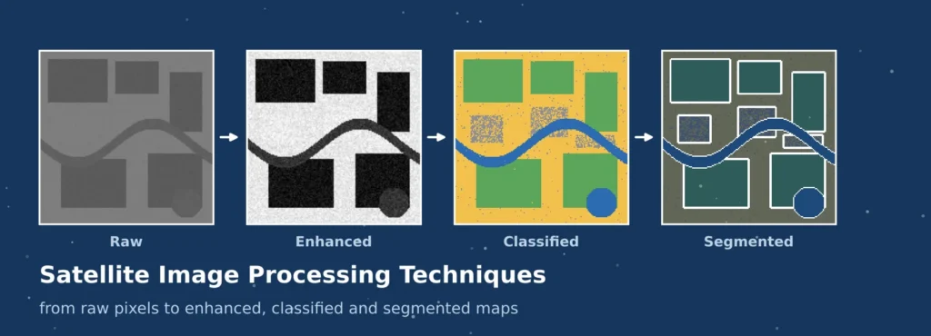
A satellite image is NOT a photograph. Is a matrix of values, one value for each pixel for each spectral band, created by a sensor which was influenced by the atmosphere, the azimuth and elevation angle of the sun, and the terrain and the sensor’s own electronics. These numbers need to be corrected, improved for interpretation, outlined into meaningful classes, and compared with reality before they can respond to a question about crops, floods or cities. That is precisely what the processing techniques of satellite imagery offer.
Things have been moving in the field very quickly. Most operational maps are still based on classical statistics, and deep learning today is used to detect buildings, roads and field boundaries on the continental scale. This guide is for both ends. It covers the most important remote sensing image processing techniques in practice: pre-processing, satellite image enhancement techniques, satellite image classification techniques and satellite image segmentation using deep learning. For an introduction into the physics see the Royal Meteorological Society primer on remote sensing.
READ MORE: Machine Learning in GIS: Applications, Tools And Use Cases
Foundations of Satellite Image Processing
Satellite images are not photographs. It is a matrix of numbers, each number corresponding to a pixel on one of the spectral bands, generated by a sensor that was impacted by the atmosphere, the sun angle, the terrain and the sensor electronics. These numbers need to be corrected; they need to be enhanced for interpretation; they need to be organized into a meaningful class or outline; they need to be tested against the real world before they can answer a question about crops, floods or cities. Satellite image processing techniques provide just that sequence.
There has been a rapid development in this field. Many maps are still based on classical statistics, and deep learning is now used to extract buildings, roads and field boundaries at the continental scale. This guide is for both ends. It covers remote sensing image processing methods that are most useful in practice: pre-processing, satellite image enhancement techniques, satellite image classification techniques, and satellite image segmentation based on deep learning. A brief introduction to the physics underlying the topic is available in the Royal Meteorological Society primer on remote sensing.
READ MORE: Advanced Remote Sensing And Satellite Imagery Services
| Stage | Purpose | Typical methods |
| Pre-processing | Make pixel values physically meaningful and correctly located | Radiometric calibration, atmospheric correction, orthorectification, cloud masking |
| Enhancement | Improve visual interpretation or highlight features | Contrast stretching, filtering, band ratios, principal components, pan-sharpening |
| Classification | Assign each pixel or object to a category | k-means, Random Forest, support vector machines, object-based analysis |
| Segmentation | Outline individual features or label every pixel by class | U-Net, DeepLab and transformer models |
| Validation | Measure reliability against independent reference data | Error matrix, IoU, F1 score, field checks |
Pre-Processing: Preparing Imagery for Analysis
Pre-processing is among the least glamorous and most crucial among all the remote sensing image processing techniques. Translates raw digital numbers into values that can be compared over time, between sensors and locations. The most common reason for two analyses of the same area to disagree is that one has been missed.
| Step | Problem it solves | Common techniques |
| Radiometric calibration | Digital numbers depend on the sensor, not the surface | Apply gain and offset to obtain radiance or top-of-atmosphere reflectance |
| Atmospheric correction | Gases and aerosols scatter and absorb light, causing haze | Dark object subtraction, radiative transfer models, Sen2Cor, LaSRC |
| Geometric correction | Pixels are displaced by sensor angle and terrain | Ground control points, orthorectification with a DEM, co-registration |
| Cloud and shadow masking | Contaminated pixels distort every later result | Fmask, s2cloudless, quality bands, compositing |
| Mosaicking and resampling | Study areas span several scenes of differing brightness | Seamline selection, histogram matching, resampling to a common grid |
Analysis ready surface reflectance products are now available from many providers. These save effort, but it is important to read the documentation as masking rules and correction models vary among providers, and discrepancies between datasets may be interpreted as a ground truth change. It is only at this stage that the use of satellite image enhancement techniques and the later stages is reliable.
READ MORE: GIS Remote Sensing Services for Accurate Mapping
Satellite Image Enhancement Techniques
Satellite image enhancements are methods used to alter the appearance, or extract information, that is difficult to extract from an image, and that can be more useful to an analyst or algorithm. The sensor has to be able to capture all the levels from dark water to bright sand and a typical scene only utilizes a small portion of the available brightness range. Four popular methods of enhancement are applied to a synthetic hazy scene, and the numbers below were computed on this scene.
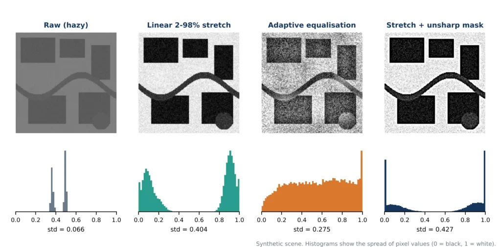
Figure 1: Four enhancements applied to a synthetic hazy scene, with the histogram of each result.
Contrast Stretching
A linear stretch rescales the range of values that is displayed to the full range of display, typically by trimming a small percentage of the extremes. For the demonstration, the raw band was between 0.33 and 0.53 on the 0 to 1 scale with a standard deviation of 0.066. Following a 2-98 spread, the spread widened to 0.404, and land cover boundaries were apparent. The percentile and standard-deviation stretches are the workhorse stretches, since they are predictable, and they are also reversible to display.
Histogram Equalisation and Adaptive Methods
Histogram equalisation redistributes brightness to use up each brightness class approximately equally in scenes that are heavily dominated by one brightness class. This is done locally in small tiles, and is called contrast-limited adaptive histogram equalisation (CLAHE). It displays texture in dark or bright regions but on the other hand, like the third panel demonstrates, it amplifies noise in uniform regions so its limit should be set conservatively.
Spatial Filtering
Filters work on neighbourhoods of pixels. Smooth noise with low pass filtering: mean, Gaussian and median smooth noise; median smooth noise preserves better edges. High-pass and edge filters such as Sobel and Laplacian highlight edges. In the fourth panel, unsharp masking was used to highlight detail by removing a fuzzy copy, with a significant increase in the spread (0.427) and tightened field edges, but a stronger accentuation of noise. Specialized speckle filters are common, such as the Lee filter, for radar images.
Band Ratios, Indices and Transformations
Combine bands to reduce illumination effects and highlight a property. The NDVI = (NIR − Red) / (NIR + Red), while water, moisture and built-up indices are similarly defined using other bands. The tasselled cap transformations are brightness, greenness and wetness; they express the information; Principal component analysis puts correlated bands into a few uncorrelated ones, concentrating the information and reducing the noise.
Pan-Sharpening
Pan-sharpening is a technique that combines a coarse multispectral image with a panchromatic image into one finer image. For example, Landsat 8 is able to fuse the 15 m panchromatic band with its 30 m colour bands. Intensity-hue-saturation, Brovey, principal component and Gram-Schmidt methods have different characteristics of preserving colour. This produces a great image for visual interpretation, but the values are altered in the spectrum and the sharpened images are not good for indices for quantitative purposes.
Satellite Image Classification Techniques
Satellite image classification techniques assign each pixel, or each group of pixels, to a category such as water, vegetation, built-up land or bare soil. They fall into three families.
- Unsupervised classification groups pixels by spectral similarity, using methods such as k-means or ISODATA, and the analyst names the clusters afterwards. It needs no training data and suits exploration.
- Supervised classification learns from labelled training samples. Maximum likelihood is the classical method, while Random Forest and support vector machines cope well with many bands and moderate sample sizes.
- Object-based image analysis first segments the image into homogeneous objects and then classifies them using colour, shape, texture and context, which reduces the salt-and-pepper effect of pixel-by-pixel methods in very-high-resolution images.
Figure 2 compares the first two on a synthetic four-band scene with four classes. The supervised Random Forest was trained on 800 pixels from the left 35 percent of the map, and both results were scored on the area outside the training strip. The unsupervised result was matched to the reference classes automatically. The scene and its accuracies come from a simulation made for this article.
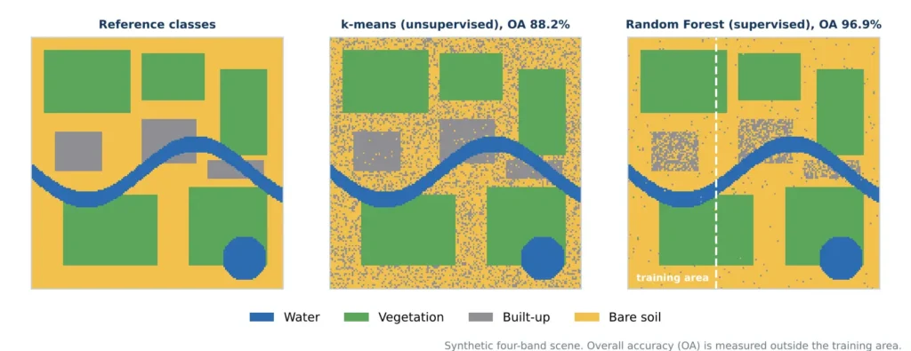
Figure 2: Unsupervised and supervised classification of a synthetic scene (overall accuracy outside the training area).
| Measure (test area) | k-means | Random Forest | Difference |
| Overall accuracy | 88.2% | 96.9% | 8.7 points |
| F1 score, built-up | 0.49 | 0.70 | 0.21 |
| F1 score, bare soil | 0.86 | 0.97 | 0.11 |
Two lessons follow. Supervised learning won because the labels told the model which spectrally similar classes to separate, and the biggest gains came for built-up land and bare soil, whose spectra overlap. And overall accuracy hides the weak class: built-up land scored far below the others even in the better model. Training samples must be well spread across each class, independent of the test samples, and checked against reliable reference data.
Satellite Image Segmentation Using Deep Learning
Satellite image segmentation using deep learning goes beyond spectral values and learns shapes, textures and context directly from labelled images. Semantic segmentation assigns a class to every pixel. Instance segmentation also separates individual objects, such as each building in a dense block. These models produce building footprints, road networks, crop field boundaries, water masks and burn scars.
The Encoder-Decoder Idea
Most models follow the pattern in Figure 3, popularised for images by U-Net. An encoder repeatedly applies convolutions and pooling, which shrinks the image while learning increasingly abstract features. A decoder then upsamples back to the original resolution. Skip connections pass fine spatial detail from encoder to decoder, which keeps the object boundaries sharp.
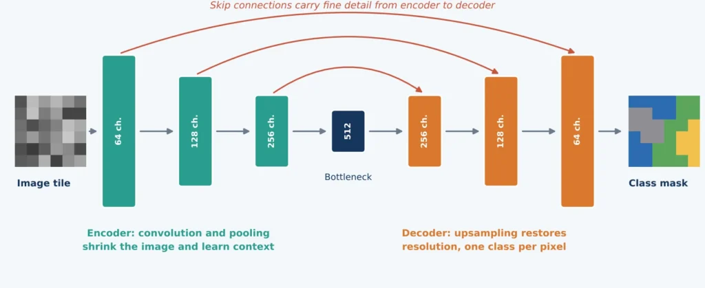
Figure 3: A simplified U-Net style encoder-decoder with skip connections.
Other widely used architectures include DeepLab, which uses dilated convolutions to see wider context, high-resolution networks that keep detail throughout, and transformer-based models that capture long-range relationships across a tile. General-purpose promptable models such as the Segment Anything Model are also being adapted to satellite imagery, mainly to speed up the creation of labels.
Training Practice
- Tiling. Large scenes are cut into tiles, commonly 256 or 512 pixels square, often with overlap so that predictions can be blended at the edges.
- Normalisation. Each band is scaled consistently, using the same statistics in training and prediction.
- Augmentation. Flips, 90-degree rotations and mild brightness changes add variety, and suit overhead imagery because it has no fixed up direction.
- Loss functions. Cross-entropy is standard, while Dice and focal losses help when the target class, such as buildings, covers only a small fraction of pixels.
- Transfer learning. Starting from pretrained weights reduces the labelled data required and speeds training.
- Metrics. Intersection over union is true positives divided by the sum of true positives, false positives and false negatives. The Dice or F1 score is twice the true positives divided by twice the true positives plus the false positives and false negatives.
Public benchmarks such as SpaceNet, DeepGlobe, the ISPRS Potsdam and Vaihingen sets and LoveDA allow methods to be compared, though a good benchmark score does not guarantee good performance on a new region. After prediction, tiles are stitched, probabilities are thresholded, and masks are converted to vector polygons, often with a regularisation step that squares building outlines and removes slivers.
Change Detection and Time-Series Processing
Many applications depend on comparing dates, and the remote sensing image processing techniques above are all reused for it. Image differencing and index differencing flag large changes quickly, post-classification comparison tabulates transitions such as cropland to built-up land, and time-series algorithms fit a trajectory to each pixel to separate genuine disturbance from seasonal cycles. All of them need images of the same season, consistent correction and accurate co-registration, otherwise phenology, haze and misalignment are read as change.
Matching Technique to Objective
The right choice among satellite image processing techniques depends on the question, the imagery and the labels available. The table links common objectives to a starting method, whether that is one of the satellite image classification techniques or a deep learning model.
| Objective | Data | Core technique | Check with |
| Visual interpretation of hazy imagery | Single scene | Contrast stretch, adaptive equalisation | Visual review, histogram |
| Sharper colour imagery | Multispectral plus panchromatic | Pan-sharpening | Colour distortion, edge quality |
| Regional land cover map | Corrected multispectral composite | Random Forest or similar | Error matrix, per-class F1 |
| Buildings, roads, field boundaries | Very-high-resolution imagery | Deep learning segmentation | IoU, precision, recall |
| Land change over years | Time series of one sensor | Index differencing, trajectory analysis | Independent reference samples |
Challenges and Limitations
Every stage has limits, and satellite image segmentation using deep learning inherits all of them while adding some of its own.
- Cloud cover and haze limit optical imagery, particularly in monsoon regions, and radar or compositing may be needed.
- Mixed pixels blend several surfaces, so features smaller than a pixel are lost or misclassified.
- Label quality. Both classifiers and deep networks inherit every error in their training data.
- Domain shift. A model trained on one region, season or sensor can perform poorly on another without local fine-tuning.
- Class imbalance. Rare classes are easily ignored when only overall accuracy is optimised.
- Compute and storage. Deep learning on large archives needs graphics processors and careful data engineering.
Best Practices for Dependable Results
These habits apply to all satellite image processing techniques, from a simple stretch to a deep network.
- Correct before analysing. Use calibrated, atmospherically corrected and co-registered data.
- Keep display and measurement separate. Use enhanced images to look, and original values to compute.
- Start simple. A Random Forest baseline shows whether a deep model adds value.
- Invest in labels. Well-distributed, accurate samples improve results more than parameter tuning.
- Test on independent areas. Hold out whole regions, and report per-class metrics.
- Check transfer. Evaluate any model in a new region or season before applying it widely.
- Document the workflow. Record sensors, dates, parameters and software versions.
Points Often Misunderstood
Several beliefs about satellite image processing techniques cause avoidable errors.
- A better-looking image is not a more accurate one. Stretching and sharpening change appearance, not truth.
- Overall accuracy can hide a weak class. The built-up class in the simulation shows how.
- Deep learning is not always the answer. With few labels and coarse imagery, classical methods can match it at lower cost.
- Pan-sharpened images are not ideal for indices. Their spectral values have been altered.
- Benchmark scores do not transfer automatically. Local testing is always needed.
Conclusion
The processing techniques of the satellite images represent one link in the chain, and the remote sensing image processing techniques discussed here are most effective in combination. Pre-processing renders the values in the pixel level trustworthy, enhancement renders the values visible, classification and deep learning segmentation results in maps and outlines, and validation reveals how reliable are the results. The most reliable projects keep the original measurements from the enhanced copies and match the method used to the purpose of the project; accuracy for each class is reported, as well as for the entire map.
For field-based training data, see our guides to GIS data collection and GIS survey services. Simbi Labs India supports research and projects that need geospatial analysis and mapping. Visit our contact page, book an appointment or reach us on WhatsApp.