
GIS and Remote Sensing Techniques for Advanced Geospatial Data Analysis
From pixels to decisions: a practical, method-driven guide
By itself, a satellite image is just a matrix of numbers. A map layer is a collection of shapes and attributes within the map. The real magic seems to occur when the two come together: pixels become measurements and those measurements appear on a map and can be compared against the boundaries, roads, rivers and population. GIS and remote sensing are utilized in conjunction in land management, agriculture, water resources, disaster mitigation and urban development, because of this.
It covers the main methods in the sequence they are encountered in a real project: selection of data, pre-processing, extraction of indices, classification, change detection and interpretation of results in a GIS. It covers a small worked example, explains the role that remote sensing can play in environmental monitoring, outlines the errors commonly encountered and how to avoid them, and more.
READ MORE: Machine Learning in GIS: Applications, Tools And Use Cases
1. How GIS and Remote Sensing Fit Together
The information about the earth’s surface is obtained from a remote distance, typically from satellite, aircraft or drone. The energy reflected and/or emitted by the ground is measured by the sensors in a number of different wavelength bands, with each band constituting a layer of values. Geographic information system (GIS) is a system used to store, manage and analyze spatial data. To sum up, remote sensing provides the data for the observations while GIS provides the context and decision ready results.
Two data models
Most of the confusion between the two fields disappears once the underlying data models are clear.
- Raster data is a regular grid of cells, each holding a value. Satellite images, elevation models and classification maps are rasters. Rasters suit continuous phenomena such as reflectance, temperature or height.
- Vector data describes features as points, lines and polygons with attributes. District boundaries, roads, well locations and field parcels are vectors. Vectors suit discrete objects with names and attributes.
Much of the analytical power comes from moving between the two, for example summarising a raster inside vector polygons (zonal statistics), or converting a classified raster into polygons for reporting.
Four kinds of resolution
Every image is a compromise between four properties, and the right choice depends on the question being asked.
- Spatial resolution is the ground size of one pixel. It limits the smallest feature that can be detected.
- Spectral resolution is the number and width of bands. More and narrower bands allow finer discrimination between materials.
- Temporal resolution is the revisit interval. It decides whether a rapid event, such as a flood or a crop growth stage, can be captured.
- Radiometric resolution is the sensitivity of the sensor to small differences in energy, expressed in bits. Higher values capture subtler contrasts.
A typical workflow
The imagery is corrected and processed, features and changes are extracted, and the corrected features are entered into a GIS for measurement, overlay and mapping. Next, the data collected in the field (e.g., GPS or survey data) is compared to ensure the results are correct. It is important to consider validation as an integral part of the workflow, not an optional extra, to distinguish a convincing analysis from a colourful map.
2. Choosing the Right Data
The first decision is which data to use. Detail, revisit time, sensor type and archive length all matter, and no single source is best for everything. The figures below are typical values; check each provider’s current documentation before planning a project.
| Data Source | Typical Detail | Best For |
| Landsat 8 and 9 | 30 m multispectral, 15 m panchromatic, thermal bands; 16-day revisit per satellite (8 days combined); continuous Landsat archive back to the 1980s | Long-term land cover and change studies, thermal analysis |
| Sentinel-2 | 10, 20 and 60 m multispectral including red-edge and SWIR bands; revisit of about 5 days with two satellites | Vegetation, crop and land use mapping at field scale |
| Sentinel-1 (radar) | C-band synthetic aperture radar; works through cloud and at night; revisit of roughly 6 to 12 days depending on region | Flood mapping, surface change and monitoring in cloudy regions |
| MODIS and similar | 250 m to 1 km; near-daily coverage | Regional drought, fire and seasonal trends |
| Drone imagery | Centimetre-level detail over small areas, flown on demand | Site surveys, local validation and very high-detail mapping |
| Digital elevation models | Roughly 30 m global products such as SRTM and Copernicus DEM; finer from LiDAR or drones | Slope, drainage, watershed and flood-risk analysis |
There are three practical rules to follow while choosing data. First, match the size of the pixels with the smallest feature of interest – a good rule of thumb is for a feature to cover several pixels, or be more likely to be detected. Second, synchronize revisit time with the process: frequent imagery is required for seasonal crop monitoring, and for decadal change of land cover it is not. Third, decide on the kind of sensor to use depending on the conditions of use: optical sensors can not be used when there is cloud, whereas radar can be used but it is more difficult to interpret.
3. Core GIS and Remote Sensing Techniques
The techniques below form the working toolkit for most projects. Together they make up the practical remote sensing data analysis techniques that teams use in desktop GIS, cloud platforms or Python.
3.1 Pre-processing
Raw sensor data is not ready for analysis. Pre-processing makes pixel values physically meaningful and comparable across space and time.
- Radiometric calibration converts raw digital numbers to radiance or top-of-atmosphere reflectance.
- Atmospheric correction removes the effects of scattering and absorption to produce surface reflectance, so that a pixel measured in summer can be compared with one from winter.
- Geometric correction aligns the image to the ground. Orthorectification uses elevation data to remove distortion from terrain, and co-registration ensures that images from different dates overlay precisely.
- Cloud and shadow masking removes contaminated pixels. Quality bands supplied with the product are the usual starting point.
- Compositing and gap filling combine several dates, for example by taking the median of clear observations over a season, to produce a clean, representative image.
Many projects now begin from analysis-ready surface reflectance products, which have already been through most of these steps. Even so, it is good practice to check the processing level and the cloud mask before trusting the data.
3.2 Spectral indices
A spectral index combines bands in a simple formula to highlight a feature and suppress unwanted variation such as illumination differences. The table lists common indices; all assume surface reflectance inputs.
| Index | Formula | Used To Highlight |
| NDVI | (NIR − Red) / (NIR + Red) | Vegetation vigour and cover |
| EVI | 2.5 × (NIR − Red) / (NIR + 6 × Red − 7.5 × Blue + 1) | Vegetation in dense canopies, where NDVI saturates |
| NDWI | (Green − NIR) / (Green + NIR) | Open water |
| MNDWI | (Green − SWIR) / (Green + SWIR) | Open water, with better suppression of built-up noise |
| NDMI | (NIR − SWIR) / (NIR + SWIR) | Vegetation moisture content |
| NBR | (NIR − SWIR) / (NIR + SWIR), using the long-wave SWIR band | Burned areas and burn severity |
| NDBI | (SWIR − NIR) / (SWIR + NIR) | Built-up surfaces |
Indices are fast, transparent and easy to explain, but they have limits. NDVI tends to saturate over dense vegetation, soil background affects sparse canopies, and built-up and bare surfaces can confuse water and urban indices. Always inspect the results visually and consider combining indices rather than relying on one.
3.3 Image classification
Classification sorts pixels into classes such as water, vegetation, built-up and bare land. The main approaches are:
- Unsupervised classification groups pixels by spectral similarity without training data, and the analyst labels the clusters afterwards. It is useful for exploration.
- Supervised classification learns from training samples marked by the analyst. Machine learning methods such as random forest and support vector machines are widely used because they cope well with many bands and non-linear class boundaries.
- Object-based image analysis groups neighbouring pixels into segments first and then classifies the segments using shape, texture and context as well as colour. It often works better on high-resolution imagery.
- Deep learning uses convolutional and transformer networks to learn spatial patterns directly, and is effective for features such as buildings, roads and field boundaries when enough labelled data is available.
Good training data matters more than the choice of algorithm. Samples should be representative of each class across the whole study area, balanced enough that small classes are not swamped, and kept separate from the samples used for testing.
Accuracy assessment
Modeling is a classified map, and the quality of the model needs to be measured. The traditional method is to gather independent reference data points (preferably via stratified random sampling to ensure that rare classes are sampled) and then compare them with the map in a confusion matrix. From this, report the overall accuracy, how much of each real class was captured (producer’s accuracy), and how reliable each mapped class is (user’s accuracy). Report intervals where applicable and never use just a single headline percentage.
3.4 Change detection
Change detection compares two or more dates to find what has changed. Common approaches include:
- Image or index differencing, which subtracts one date from another and applies a threshold. It is simple and effective, as the worked example below shows.
- Post-classification comparison, which compares two classified maps and produces a from-to matrix, for example forest to cropland. Errors in either map compound in the result.
- Time-series analysis, which fits trends and detects breakpoints across many dates, separating genuine disturbance from seasonal cycles and noise. Methods such as LandTrendr, BFAST and CCDC are widely used for this.
Whatever the method, change maps should be filtered with a minimum mapping unit to remove isolated pixels, and compared across the same season so that phenology is not mistaken for land change.
3.5 Spatial analysis in GIS
With the features and changes extracted, GIS translates them into answers. Overlay merges layers, buffer calculates distance to assets and proximity finds the distance from assets, and zonal statistics summarises raster values within polygons. For instance, a change map could be used to determine how many hectares of lost vegetation are occurring within each district, how many homes are within 500 metres of an area burned, or the distance of road open to flood. Area or distance calculations should be in an appropriate projected coordinate system and not in latitude and longitude.
3.6 Terrain and elevation analysis
Slope, aspect, curvature, flow direction and flow accumulation and watershed delineation are supported by digital elevation models. With imagery, they help to describe why patterns exist: vegetation stress on south facing slopes, spread of flooding in low lying areas, or erosion potential on steep hills with cleared vegetation. Terrain correction also improves the quality of radar and optical imagery in mountainous areas.
4. Why Spectral Indices Work
Red light is absorbed in the leaf for photosynthesis and near-infrared light is heavily scattered within the leaf. The outcome is a distinct increase in reflectance in the red edge region (between the red band and the near infrared band). The soil is devoid of vegetation and slopes upward across the spectrum, while water has a strong absorption in the infrared. An index like NDVI takes advantage of the difference between the red and near-infrared: values close to 1 are associated with dense, healthy vegetation; values around 0 are associated with bare surfaces; negative values are typically associated with water or cloud. This idea is sketched in a schematic way as curves in figure 1.
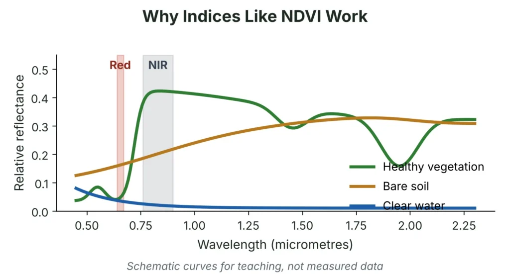
Figure 1: Schematic reflectance of vegetation, bare soil and water (for teaching only).
5. A Worked Example: Detecting Vegetation Loss
To show the logic, a small synthetic scene was created with two dates. Between the dates, one patch of vegetation was converted to bare ground and the edge of a built-up area was expanded. NDVI was calculated for each date and the difference was mapped. Pixels that were vegetated on the first date and lost more than 0.25 NDVI units were flagged as loss.
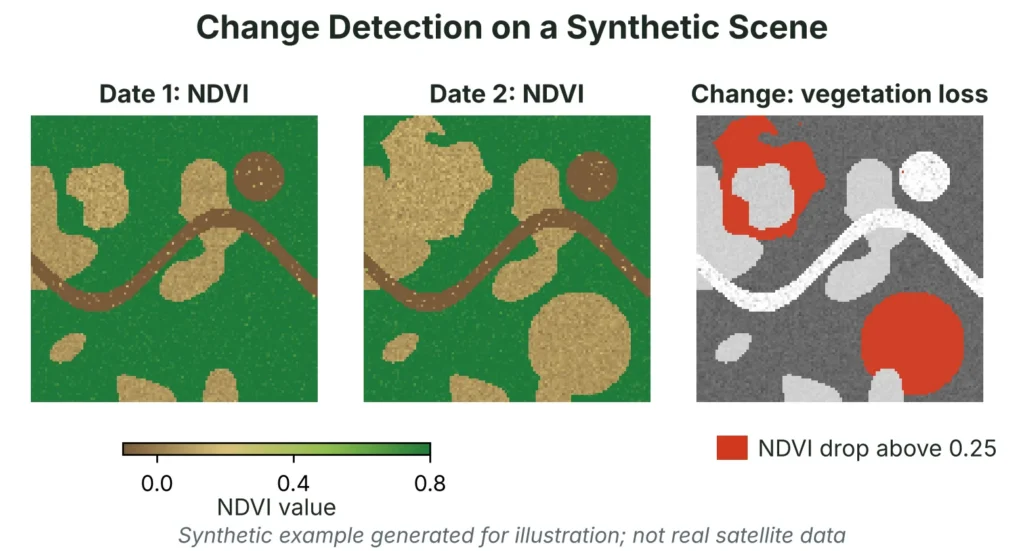
Figure 2: NDVI for two dates and the resulting loss map (synthetic scene, illustrative only).
In this example the share of the scene with NDVI above 0.4 fell from about 72% to about 55%, and about 17.5% of the scene was flagged as vegetation loss. These numbers describe the invented scene and carry no real-world meaning. What matters is the method: a vegetation threshold on the first date, a drop threshold between dates, and a map of the result.
In a real project the same logic needs several additional safeguards:
- Apply a cloud and shadow mask to both dates.
- Compare images from the same season, and preferably the same sensor.
- Test the thresholds against reference data instead of accepting defaults.
- Remove small isolated patches using a minimum mapping unit.
- Validate with field or high-resolution reference points and report the accuracy.
- Summarise the loss by district or zone in GIS and present it with clear maps.
6. Remote Sensing in Environmental Monitoring
Remote sensing is valuable in environmental monitoring because it gives repeated, consistent coverage of large and hard-to-reach areas, and builds a record that can be revisited. Combined with GIS, it turns observations into maps and statistics that agencies and communities can act on. The table shows common questions and how they are approached.
| Environmental Question | Typical Remote Sensing Approach | GIS Contribution |
| Is forest cover shrinking? | NDVI or classification compared across dates; time-series breakpoint detection | Area statistics by district or protected zone |
| Where has a fire burned? | NBR before and after the fire, differenced to estimate burn severity | Overlay with settlements, roads and land ownership |
| Is a reservoir changing? | Water index mapped over time, or radar for cloudy seasons | Shoreline area and catchment context |
| Where is a flood spreading? | Radar imagery compared with a dry baseline | Exposure of homes, farms and roads |
| Is a city getting hotter? | Thermal bands combined with land cover and vegetation cover | Link to wards, parks and building density |
| Is a crop season on track? | NDVI time series against past seasons | Zonal summaries by field or block |
| Is land degrading or eroding? | Vegetation trends, bare soil indices and terrain analysis | Slope, soil and land-use overlays |
Each of these applications depends on the same discipline: use suitable data, process it consistently, and check results against ground truth. Remote sensing shows patterns reliably, but explaining why they occur usually needs local knowledge, field evidence and often other datasets such as rainfall, policy records or economic data.
READ MORE: Powerful Environmental Remote Sensing and GIS Solutions
7. Common Problems and How To Avoid Them
| Common Problem | Why It Matters | What To Do |
| Comparing images from different seasons | Natural phenology looks like change | Use the same time of year, or model seasonality in a time series |
| Cloud and shadow left in the data | Produces false loss and false water | Apply cloud masks, composite several dates, or use radar |
| Mixed coordinate systems | Layers misalign and areas are miscalculated | Reproject everything to one suitable projected system |
| Using raw pixel values | Values are not comparable across dates or sensors | Use calibrated surface reflectance products |
| Mixed pixels at coarse resolution | One pixel holds several land covers | Use finer imagery, or unmix or report results as fractions |
| Imbalanced or biased training samples | Rare classes are missed and accuracy is overstated | Sample representatively and balance classes |
| Testing on training data | Gives falsely high accuracy | Hold out independent, spatially separate reference points |
| Radar speckle and terrain effects | Noise and geometric distortion | Filter speckle and apply terrain correction |
| No ground check | Errors go undetected | Validate with field points or higher-resolution imagery |
8. Quality, Uncertainty and Reproducibility
The geospatial results are not facts, but estimates, and it is good to present them as such, as this fosters trust. Document the data sources, dates, processing steps, parameters and versions of software used so that it can be repeated or revised. Accurately report uncertainty and error with each map and statistic and be careful with area figures; small differences in area classification accuracy can overwhelm small differences on the ground. Include metadata with each layer, and save the workflow as a series of documents and recorded models, not as a bunch of unrecorded clicks.
9. Tools and Platforms
This guide demonstrates how to use various tools to perform the techniques. The Desktop GIS (QGIS and ArcGIS Pro) enables visual analysis, classification and cartography. Time-series analysis can benefit from large archive and quick processing of cloud platforms like Google Earth Engine. Reproducible, scripted workflows are possible with Python libraries such as GDAL, rasterio, GeoPandas and scikit-learn, while ESA’s SNAP toolbox is a common radar processing tool. This selection is dependent on the size of the project, the skill level of the team and the desire for repeatability.
10. A Practical Project Checklist
- Define the question. Decide exactly what must be measured, over what area and period, and the accuracy needed.
- Pick data. Match resolution, revisit time and sensor type to the feature and the timescale.
- Process consistently. Use calibrated data, one coordinate system and cloud masks.
- Extract and classify. Apply indices or classification and record every setting.
- Validate. Check results against independent field points or finer imagery and report accuracy.
- Map and report. Use GIS to summarise by area, state the uncertainty and present clear maps.
GIS and Remote Sensing Support From Simbi Labs
Simbi Labs offers GIS survey services that support geospatial analysis for planning and monitoring projects. Explore the service page, or book a free consultation to discuss your project.
Frequently Asked Questions
1. What are GIS and remote sensing techniques?
They are methods for collecting imagery of the Earth, extracting information such as land cover or change, and analysing the results in a GIS alongside other map data such as boundaries, infrastructure and population.
2. What are the main remote sensing data analysis techniques?
Pre-processing, spectral indices, image classification, change detection and time-series analysis, usually followed by spatial analysis in GIS and an accuracy assessment.
3. How is remote sensing used in environmental monitoring?
It is used to track forest cover, burned areas, water bodies, floods, urban heat and crop condition across large areas and over time, giving consistent evidence for planning and response.
4. Why use GIS together with remote sensing?
Remote sensing detects what is on the ground, while GIS adds boundaries, assets and population data, so image results can be summarised by area and used in decisions.
5. Which satellite data should I start with?
For most land and vegetation work, Sentinel-2 offers a good balance of detail and revisit, and Landsat provides a long archive for historical change. Use Sentinel-1 radar when cloud is a problem.
6. How accurate are classified maps?
It depends on the data, classes and training samples. Always measure accuracy with independent reference points and report producer’s and user’s accuracy for each class, not just an overall figure.