
Paired T-Test: Formula, Examples, Assumptions, Interpretation & SPSS

Understanding the Paired t-Test and Its Statistical Purpose
A paired t test—sometimes called a dependent t test or paired samples t test—is a statistical method used to analyze whether there is a significant difference between the means of two related sets of observations.
Unlike the independent t test, which compares the means of two distinct groups (e.g., males vs. females, treatment group vs. control group), the paired t-test is designed for situations where the same individuals or matched subjects are measured twice. These two measurements are “paired” because they come from the same source, making them dependent rather than independent.
A paired t-test is a statistical test used to determine whether the mean difference between two related measurements is statistically significant. It is commonly used when the same participants are measured twice, such as before and after an intervention.
For example, if 10 students take a test before and after a training program, a paired t-test can determine whether their average scores changed significantly.
The test is based on the difference between each pair of observations:
Difference = Second Measurement − First Measurement
The paired t-test then evaluates whether the mean difference is significantly different from zero.
Why is this important?
One major strength of the paired t-test is that it controls for individual differences. By comparing each subject with themselves, the paired design accounts for between-subject variability that would otherwise contribute to the comparison. The analysis focuses on the within-subject differences, which can improve statistical efficiency when the pairing is appropriate.
Common Applications of the Paired t test
The paired t-test can be used across many fields when two measurements are related or come from the same subjects.
| Field | Example of Paired Data |
| Medical Research | Blood pressure before and after treatment |
| Education | Test scores before and after a teaching method |
| Business Analytics | Employee productivity before and after training |
| Psychology | Stress scores before and after an intervention |
| Sports Science | Athlete performance under two conditions |
| Environmental Research | Measurements taken at two related locations or conditions |
Identifying the Right Situation for a Paired T-Test
The paired t-test is most suitable in situations where the two sets of data are related rather than independent. This relationship typically arises when the same individuals are measured twice, or when subjects are matched in a meaningful way. The goal is to evaluate whether the observed differences between the paired values are statistically significant.
Here are the most common scenarios where a paired t-test is appropriate:
1. Before-and-After Studies
This is the most widely used application of the paired t-test. The same subjects are measured before and after an intervention, allowing researchers to determine if the intervention caused a significant change.
Medical Example: Measuring patients’ blood pressure before they start medication and again after completing the treatment.
Educational Example: Comparing student scores on a pre-test and post-test to evaluate the effectiveness of a new teaching strategy.
Business Example: Tracking employee productivity before and after implementing new software.
2. Two Conditions on the Same Subjects
Sometimes, the same group of individuals is tested under two different conditions. Since each subject serves as their own control, the paired t-test is ideal for analyzing whether condition A and condition B produce different outcomes.
Sports Example: Measuring athletes’ reaction times with caffeine intake vs. without caffeine.
Psychology Example: Evaluating stress levels in participants during a quiet environment vs. a noisy environment.
3. Matched Pairs Design
In some studies, participants are not identical but are matched based on key characteristics (e.g., age, gender, or background). Each pair is then split into two groups—one receives the treatment, while the other does not. The similarity between matched individuals helps control for external variability.
Example in Twin Studies: Comparing identical twins where one twin receives a new treatment and the other serves as the control.
Sociology Example: Pairing employees with similar job roles to test the impact of different training programs.
4. Naturally Paired Data
Sometimes, data are naturally paired because of a physical or logical connection between the observations. In such cases, each observation in one group has a direct counterpart in the other group.
Medical Example: Comparing grip strength in a person’s dominant (right) hand vs. non-dominant (left) hand.
Environmental Example: Measuring pollutant levels in river water upstream vs. downstream at the same location.
The Key Criterion
In all these scenarios, the critical requirement is that the data are paired or related, not independent. Each observation in one group must have a meaningful link to a corresponding observation in the other group. This dependency is what makes the paired t-test the correct choice instead of the independent t-test.
Paired T-Test vs Independent T-Test
The main difference between a paired t-test and an independent t-test is the relationship between the observations.
| Feature | Paired T-Test | Independent T-Test |
| Observations | Related or dependent | Independent |
| Participants | Same or meaningfully matched subjects | Different subjects |
| Main comparison | Mean within-pair difference | Difference between group means |
| Typical design | Before-and-after | Treatment vs control |
| Example | Pre-test vs post-test scores | Group A vs Group B scores |
Example
Suppose 30 students complete a test before and after a training program. Because the same students are measured twice, the observations are paired and a paired t-test may be appropriate.
Now suppose 30 students in Group A are compared with a different 30 students in Group B. Because the observations come from different, unrelated groups, an independent-samples t-test may be appropriate.
Therefore, the choice between the two tests depends primarily on the study design and relationship between observations, not simply on the number of groups.
Assumptions
Like all statistical tests, the paired t-test relies on certain assumptions to ensure that the results are valid and interpretable. Violating these assumptions can lead to misleading conclusions. The three main assumptions are:
1. Independence Between Pairs
i. Each pair of observations (e.g., pre-test and post-test for one student) should be independent of all other pairs in the dataset.
ii. Example: One student’s test scores should not influence another student’s scores.
iii. This ensures that the differences you calculate within each pair are not biased by external dependencies.
2. Normality of Differences
i. The differences between the paired observations (not the raw scores themselves) should approximately follow a normal distribution.
ii. This assumption is especially important when the sample size is small (n < 30).
iii. If the sample size is large, the Central Limit Theorem allows some relaxation of this requirement, as the distribution of the mean difference will tend to approximate normality.
iv Normality can be checked using:
Graphical methods: histograms, Q–Q plots
Statistical tests: Shapiro–Wilk test, Kolmogorov–Smirnov test
3. Continuous Data (Interval or Ratio Scale)
i. The variable of interest should be measured on an interval or ratio scale, meaning the data must be numeric and represent meaningful differences.
ii. Examples: test scores, blood pressure, weight, time, or temperature.
iii. Categorical or ordinal data (like “poor,” “good,” “excellent”) are not suitable for a paired t-test.
By ensuring these assumptions hold, researchers can trust that the paired t-test will produce statistically sound results.
Formula & Hypotheses
A paired t-test is calculated using the differences between each pair of observations.
For each pair:
dᵢ = X₂ᵢ − X₁ᵢ
The mean difference is:
d̄ = Σdᵢ / n
The paired t-test statistic is:
t = d̄ / (sᵈ / √n)
Where:
- d̄ = mean of the paired differences
- sᵈ = standard deviation of the paired differences
- n = number of paired observations
- t = calculated t-statistic
The degrees of freedom are:
df = n − 1
The test compares the observed mean difference with the variability of the differences. A larger absolute t-value generally provides stronger evidence against the null hypothesis of zero mean difference.
Hypotheses
For a two-tailed paired t-test:
Null hypothesis (H₀): μd = 0
There is no population mean difference between the two paired measurements.
Alternative hypothesis (H₁): μd ≠ 0
The population mean difference is not zero.
For a one-tailed test:
H₁: μd > 0
The second measurement is expected to be greater.
H₁: μd < 0
The second measurement is expected to be lower.
How to Calculate a Paired T-Test
The calculation of a paired t-test can be understood in the following steps.
Step 1: Calculate Each Difference
For every pair of observations, calculate:
dᵢ = Second Measurement − First Measurement
Step 2: Calculate the Mean Difference
Add all difference scores and divide by the number of pairs:
d̄ = Σdᵢ / n
Step 3: Calculate the Standard Deviation of the Differences
Calculate the standard deviation using the difference scores.
Step 4: Calculate the Standard Error
SE = sᵈ / √n
Step 5: Calculate the t-Statistic
t = d̄ / SE
Step 6: Calculate Degrees of Freedom
df = n − 1
Step 7: Determine the P-Value
Use the calculated t-statistic and degrees of freedom to determine the p-value.
Step 8: Interpret the Results
Compare the p-value with the predetermined significance level, such as α = 0.05.
However, statistical significance should not be interpreted by itself. A stronger analysis also reports the mean difference, 95% confidence interval, and effect size.
Common Mistakes When Using a Paired T-Test
1. Using a Paired T-Test for Independent Groups
A paired t-test should not normally be used when the two groups consist of unrelated participants.
2. Checking Normality of the Wrong Data
For a paired t-test, the relevant normality assessment concerns the difference scores, not simply the two raw variables separately.
3. Assuming p < .05 Means the Effect Is Large
A statistically significant result does not automatically indicate a large or practically important effect. Consider the effect size and confidence interval.
4. Interpreting Correlation as Evidence of a Difference
A strong correlation between two measurements does not demonstrate that their means are significantly different.
5. Ignoring Outliers
Extreme difference scores can have a substantial influence on the mean difference and test statistic.
6. Automatically Removing Outliers
An unusual observation should not be removed simply because it affects significance. First determine whether it represents a data-entry error, measurement problem, or genuine observation.
7. Claiming Causation From a Before-and-After Comparison
A significant paired t-test demonstrates evidence of a mean change. It does not, by itself, prove that an intervention caused the change.
Step-by-Step Analysis Using SPSS

To better understand how a paired t-test works, let’s walk through a practical example.
Scenario
A teacher wants to evaluate whether a new teaching method improves student performance. She administers a pre-test before introducing the new method and a post-test afterward to the same group of 10 students. The goal is to determine if the post-test scores show a statistically significant improvement compared to the pre-test scores.
Sample Data
| Student | Pre-Test | Post-Test |
| A | 70 | 75 |
| B | 65 | 68 |
| C | 80 | 83 |
| D | 72 | 70 |
| E | 60 | 66 |
| F | 85 | 90 |
| G | 78 | 79 |
| H | 74 | 76 |
| I | 69 | 72 |
| J | 82 | 87 |
The step by step procedure to perform paired t test using SPSS is given below:
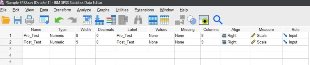
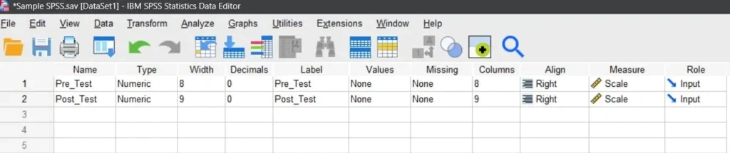
Step 1: Enter the Data in SPSS
i. In the Data View, create two columns:
Pre_Test (scores before the method)
Post_Test (scores after the method)
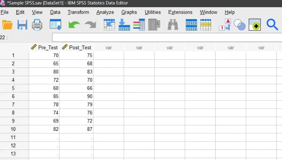
ii. Enter the values for all 10 students.
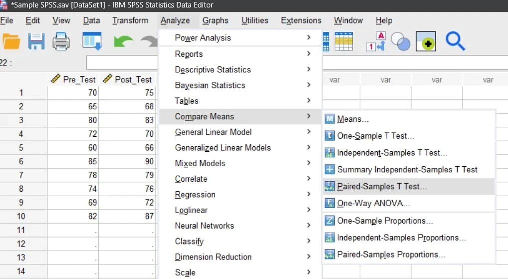
Step 2: Run the Paired t-test
- Go to the top menu and select:
Analyze → Compare Means → Paired-Samples T Test
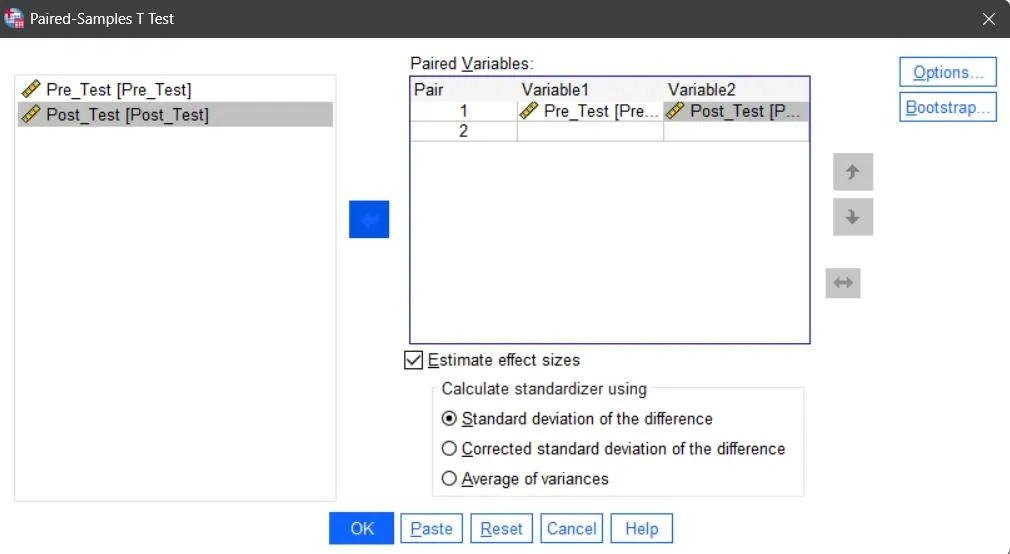
i. In the dialog box, move Pre_Test into the Variable 1 field and Post_Test into the Variable 2 field.
ii. Click OK to run the analysis.
Step 3: Review the Output
SPSS will produce several tables. Let’s interpret them step by step.
a) Paired Samples Statistics
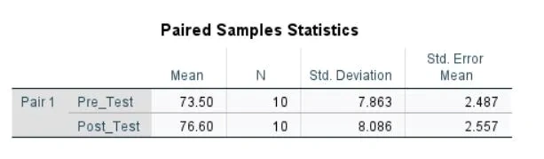
This table gives the mean and standard deviation for each condition:
Pre-Test Mean = 73.5
Post-Test Mean = 76.6
Difference = 3.1
Interpretation: On average, scores increased by 3.1 points after the new method.
b) Paired Samples Correlations
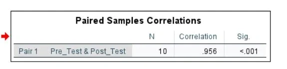
This shows the correlation between pre-test and post-test scores.
Example: Correlation = 0.95 (p < 0.001)
Interpretation: The high correlation confirms that the scores are strongly related (as expected, since they come from the same students).
c) Paired Samples Test

This is the main results table. Key columns:
Mean Difference = 3.1
Standard Deviation of Differences ≈ 2.37
t-value = 4.12
Degrees of Freedom (df) = 9
Sig. (2-tailed) = 0.003
Step 4: Make the Decision
i. The significance value (p = 0.003) is less than 0.05.
ii. Therefore, we reject the null hypothesis (H₀).
Step 5: Interpretation
We can write the interpretation of this analysis as follow”
The paired t-test results indicate a mean improvement of 3.1 points in student scores after introducing the new teaching method. The variability in these differences was relatively small (SD ≈ 2.37), and the calculated t-value of 4.12 with 9 degrees of freedom shows strong evidence against the null hypothesis.
The significance level (p = 0.003) is well below the conventional threshold of 0.05, meaning the likelihood that this improvement occurred by random chance is extremely low.
Conclusion:
The new teaching method produced a statistically significant and positive effect on student performance. In other words, students performed better after the method was introduced, and this improvement can be confidently attributed to the intervention rather than random variation.
Checking Assumptions
Before interpreting a paired t-test, confirm that its assumptions are reasonably met. Sound assumption checks protect you from false positives/negatives and make your conclusions defensible.
1) Normality of the differences (not the raw scores)
What to check: The distribution of pairwise differences (Post − Pre) should be approximately normal—roughly bell-shaped and symmetric, without heavy tails.
Why it matters: The t-test relies on normality of the sampling distribution of the mean difference. With small samples (e.g., n<30), non-normal differences can distort p-values and confidence intervals.
How to judge: Use visual diagnostics (histogram, Q–Q plot) and a normality test (Shapiro–Wilk is preferred for small samples). For moderate/large n, focus more on plots and robustness to mild deviations.
2) Outliers in the differences
What to check: Unusually large/small difference values that can drive the mean and inflate the standard error.
Why it matters: A single extreme difference can flip significance.
How to judge: Use boxplots and casewise diagnostics; verify data entry; investigate measurement/context. Outliers need transparent handling (correction if erroneous; sensitivity analysis, transformation, or robust alternative if genuine).
3) Independence between pairs
What to check: Each pair (one participant’s pre/post) is independent of other pairs.
Why it matters: Correlated pairs across subjects (e.g., classmates graded in groups, family clusters) violate the model and can bias inference.
How to judge: This is primarily a design assumption, not a statistical test. Ensure subjects/pairs were sampled independently and that no clustering requires a mixed-effects model.
4) Measurement scale
Data should be continuous (interval/ratio), e.g., time, scores, weight, BP. Ordinal/categorical data are not appropriate for a paired t-test.
Central Limit Theorem (CLT) note
With larger samples (≈ ≥30 pairs), the t-test is fairly robust to mild non-normality. Severe skew/heavy tails or influential outliers still warrant caution and possibly a nonparametric alternative (e.g., Wilcoxon signed-rank).
How to Check Assumptions in SPSS (Step by Step)
Goal: Create a difference variable, then examine its shape, outliers, and normality.
Step 1 — Compute the difference variable
i. Transform → Compute Variable…
ii. Target Variable: Diff
iii. Numeric Expression: Post_Test – Pre_Test
iv. OK
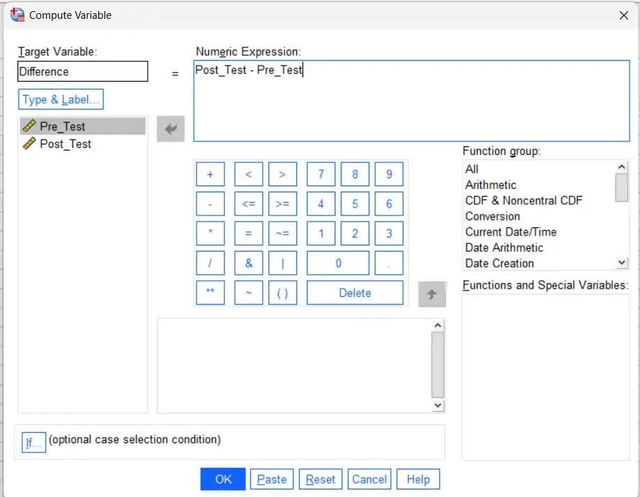
All diagnostics below use Diff.
Step 2 — Visual diagnostics (Histogram + Q–Q plot)
i. Analyze → Descriptive Statistics → Explore…
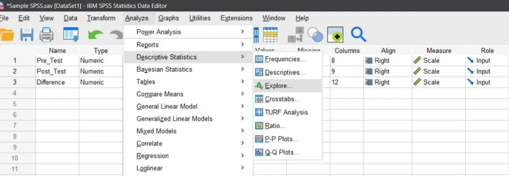
ii. Dependent List: move Diff
iii. Click Plots…
Check Histogram
Check Normality plots with tests (this gives Q–Q plot and Shapiro–Wilk)
(Optional) Under Boxplots, choose Factor levels together
iv Continue → OK
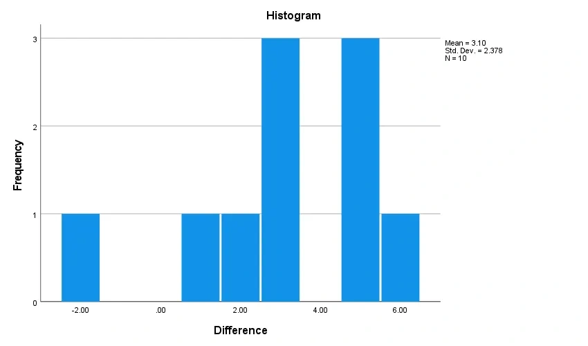
Interpretation:
Histogram: Look for an approximately bell-shaped, symmetric distribution without long tails.
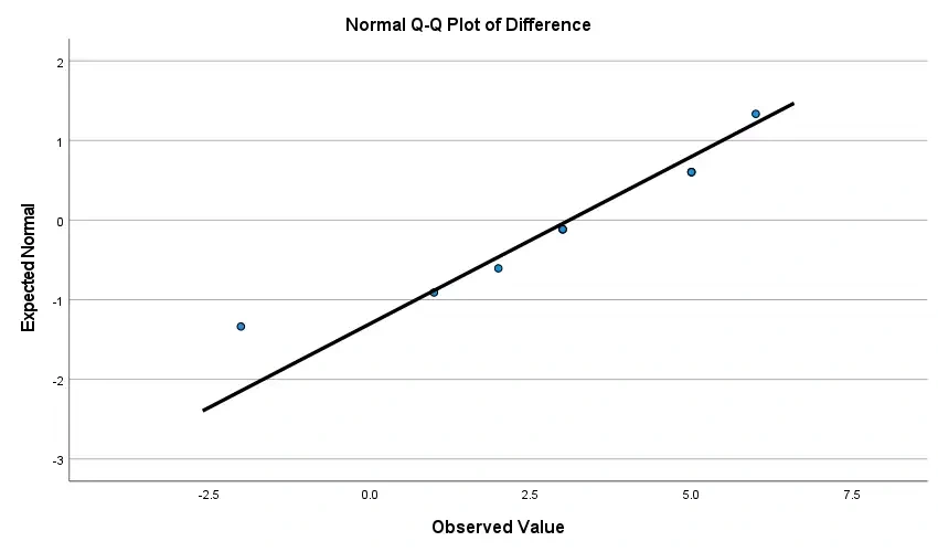
Q–Q plot: Points close to the diagonal line = acceptable. Systematic S-shapes or tail deviations suggest non-normality.
Step 3 — Formal normality test (Shapiro–Wilk)
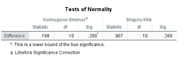
In the Explore output, find Tests of Normality.
Shapiro–Wilk p-value:
p > .05 → Fail to reject normality (normality plausible).
p ≤ .05 → Evidence against normality (inspect plots; consider remedies below).
Tip: For large n, Shapiro–Wilk can flag trivial deviations; rely more on plots and robustness.
Interpretation
Because both p-values are greater than .05, we fail to reject the null hypothesis of normality. There is no statistical evidence that the distribution of difference scores departs from normality. For a paired t-test, the normality assumption of the differences is satisfied.
Step 4 — Outlier detection
In Explore, review the Boxplot and (if shown) Casewise diagnostics.
SPSS marks mild outliers with circles and extreme outliers with asterisks.
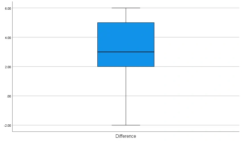
There are no outliers in the box plot.
What to Do if Assumptions Are Questionable
If normality is violated (especially with small n)
Use a nonparametric alternative:
Analyze → Nonparametric Tests → Legacy Dialogs → 2 Related Samples…
Choose Wilcoxon Signed-Rank (tick “Wilcoxon”), set Pre_Test vs Post_Test, OK.
Or transform the differences (if meaningful): log/square-root for positively-skewed strictly-positive measures; be sure the transformation is substantively defensible and re-check assumptions.
If outliers dominate the result
Justify and retain (report sensitivity analysis), winsorize (with caution), or switch to robust/nonparametric methods. Always document your choice.
If independence between pairs is doubtful
Consider design fixes (sample independently) or use models for clustered/repeated data (e.g., linear mixed-effects) rather than a paired t-test.
Software Implementation
SPSS (priority): Use the Paired-Samples T Test to analyze pre/post or matched data. SPSS outputs the mean difference, SD of differences, t, df, Sig. (2-tailed), and 95% CI. You can also report an effect size (e.g., Cohen’s dz =d/Sd ) for magnitude of change.
R: t.test(before, after, paired = TRUE) — returns the mean difference, t, df, p, and confidence interval.
Python (SciPy): scipy.stats.ttest_rel(before, after) — returns t and p; compute the mean difference, CI, and effect size from the difference vector.
Excel (Analysis ToolPak): t-Test: Paired Two Sample for Means — provides means, t, and two-tailed p; add CIs/effect size as needed.
Note: All platforms support reporting p-values, confidence intervals, and effect sizes, which together provide a clearer, more informative interpretation than p-values alone.
Summary
The paired t-test is a robust, widely used method for quantifying change within the same subjects or matched pairs. By analyzing within-person differences, it reduces between-person noise and isolates the effect of an intervention or condition.
i. In SPSS, you can run the test in minutes, obtain the mean difference, t, p-value, and 95% CI, and easily compute Cohen’s dz for effect size.
ii. When assumptions (normality of differences, independence between pairs, appropriate measurement scale) are checked and reasonably met, the paired t-test yields clear, defensible insights—making it a mainstay in medicine, psychology, education, and business analytics.
Simbi Labs recommends that whenever data are paired or matched, researchers should consider paired t-tests for more accurate inference.
For better understanding and hands-on practice, the sample dataset and SPSS output used in this analysis are also provided for reference.