Power Analysis for Univariate Linear Regression in SPSS

Introduction

Statistical power is one of the most critical, yet often overlooked, concepts in research design. If you want to build a strong foundation in statistical data analysis, check our guide on key concepts and practical tips. In simple terms, it’s your study’s ability to detect a real effect when it actually exists. Too little power, and you risk missing important findings (Type II error). Too much power, and you may waste resources collecting more data than necessary.

SPSS’s Power Analysis feature allows you to determine the right sample size before collecting data or to evaluate whether your existing study design is adequate. In this blog, we focus specifically on the “Regression – Univariate Linear” option within SPSS’s Power Analysis menu, with a special emphasis on the “Estimate power” setting.

We’ll show you how this option works, walk through the step-by-step process in SPSS, and explain how to interpret the results — using a hypothetical student dataset on Study Hours and Exam Scores so the process is crystal clear and easy to follow.

What is Univariate Linear Regression – Power Analysis?

Purpose:

To check whether a single predictor variable significantly explains variation in an outcome variable and to determine if the sample size is sufficient for detecting the expected relationship.

Example:

You want to check if study hours per week significantly predict exam scores in your class.

What is the goal of power analysis?

The goal of power analysis is to ensure that a study includes enough participants to reliably detect a meaningful effect, while avoiding the collection of more data than necessary. It strikes a balance between statistical accuracy and the efficient use of time and resources.

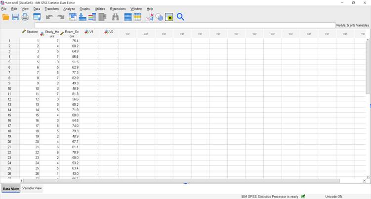
Hypothetical Dataset:

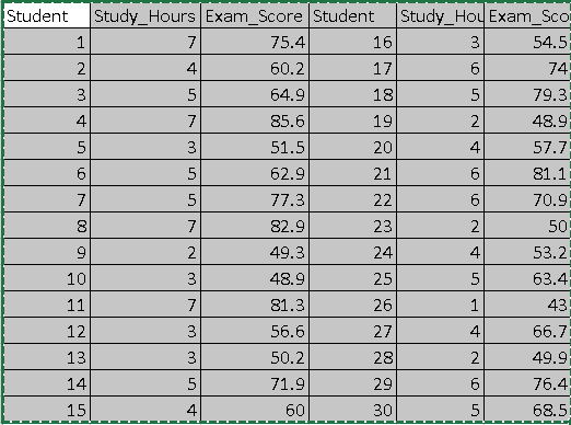
Summary of Dataset:

Multiple Partial Correlation Coefficient =0.9327

No of Test predictors = 1

Hypothesis:

i. Null Hypothesis (H₀): Study_Hours does not significantly predict Exam_Score.

ii. Alternative Hypothesis (H₁): Study_Hours significantly predicts Exam_Score.

iii. Significance Level: α = 0.05

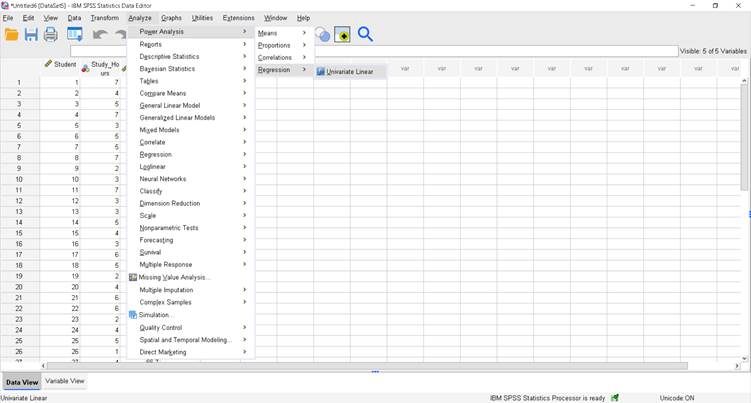
What are the steps in spss?

Step 1 – Open the Power Analysis Window

In SPSS:

Analyze > Power Analysis > Linear Regression

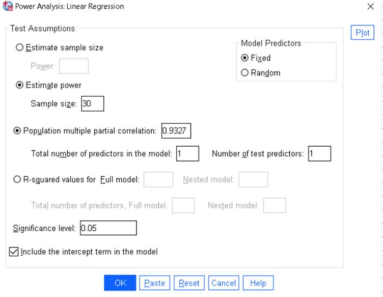
Step 2 – Enter Values for Achieved Power

Since we want to calculate the achieved power for our existing dataset:

i. Select Estimate power

ii. Sample size: 30

iii. Population multiple partial correlation: (Enter the observed Pearson correlation from your dataset)

iv. Total number of predictors: 1

v. Number of test predictors: 1

vi. Significance level: 0.05

vii. Model Predictors: Fixed

viii. Tick Include the intercept term in the model

Step 3 – Run the Analysis

Click OK.

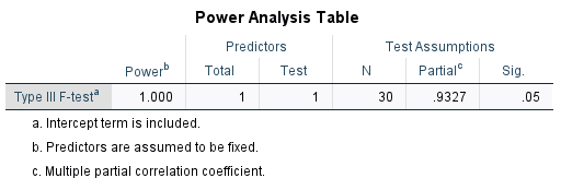
How to Write the Interpretation for Linear Regression Power Analysis in SPSS

The achieved statistical power for the Type III F-test in the linear regression model, with one predictor (Study_Hours) and an intercept term included, is 1.000 (100%). This means that with a sample size of 30, an observed multiple partial correlation of 0.9327, and a significance level of 0.05, there is virtually a 100% probability of correctly rejecting the null hypothesis if the alternative hypothesis is true. This indicates the study is extremely well-powered to detect the relationship between study hours and exam score.

For an in-depth understanding, please refer to our book, “Academic Research Fundamentals: Research Writing and Data Analysis”. It is available as an eBook here, or you may purchase the hardcopy here .