Linear Regression Basics: Simple, Multiple, Stepwise & Polynomial Models

If you’re just starting out, this overview also fits well into a longer roadmap for mastering linear regression and other key techniques—check our guide on how to learn statistical data analysis effectively.

Why Should You Care About Linear Regression?

Have you ever thought about how companies figure out how much they’ll sell next month, how banks figure out how risky a loan is, or how streaming services suggest your favourite shows? Linear regression is one of the simplest yet most effective statistical methods that may help us understand these common things. To comprehend relationships, think of it as drawing a straight line across a bunch of data points.

For example, think about how you manage your monthly budget. Your income typically tells you how much you can spend. If you make more money, you probably spend more money too. That link, which is basic, apparent, and observable, is what linear regression is based on.

In a world where there is too much data, linear regression is still a reliable guide. Even though there are better machine learning algorithms out there, this one is still popular since it’s simple to understand, works well, and gives companies useful information.

What is Linear Regression?

Choosing the right regression method depends heavily on the kind of variables you are analyzing. To refresh the basics, see our post on data types in statistics.

At its core, linear regression is about explaining or predicting one variable (called the dependent variable) using one or more other variables (independent variables).

1. Dependent Variable (Y): The outcome we want to predict (e.g., sales revenue).

2. Independent Variable (X): The factor(s) influencing the outcome (e.g., advertising spend).

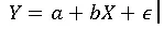
The general equation looks like this:

Where a is the intercept, b is the slope, and ε is the error term.

In business, this could mean predicting how much sales increase with every extra dollar spent on marketing or how fuel efficiency changes with car weight.

Types of linear regression

1. Simple Linear Regression: 

Predicts a dependent variable using a single independent variable. It establishes a linear relationship, allowing straightforward analysis and forecasting of trends in research or business data.

2. Multiple Linear Regression: 

Uses two or more independent variables to predict a dependent variable. Helps understand complex relationships, quantify influence of each factor, and improve accuracy in predictions and decision-making.

3. Polynomial Regression:

 Models non-linear relationships by including polynomial terms of independent variables. Captures curvature in data trends, providing better fit when simple linear models are insufficient.

4. Ridge and Lasso Regression (Regularized Regression): 

Adds penalties to regression coefficients to prevent overfitting. Ridge shrinks coefficients; Lasso can eliminate irrelevant variables, improving model stability and predictive performance in complex datasets.

5. Stepwise Regression: 

Automatically selects significant independent variables by adding/removing predictors based on statistical criteria. Optimizes model simplicity and predictive power, reducing overfitting and improving interpretability in research studies.

1. Simple Linear Regression  –  One Cause, One Effect

Simple linear regression focuses on modeling the relationship between two variables: one independent variable (X) and one dependent variable (Y). The mathematical equation is:

Where:

Y = dependent variable (what we predict).

X = independent variable (predictor).

a = intercept (value of Y when X=0).

b = slope (change in Y for every unit change in X).

ε = error term (unexplained variation).

Assumptions of Simple Linear Regression

i. The relationship between X and Y is linear.

ii. Errors are normally distributed.

iii. Errors are independent of each other.

iv. Variance of errors is constant (homoscedasticity).

Interpretation of Slope & Intercept

Slope (b): Explains the rate of change. If slope = 5, it means Y increases by 5 units for every 1 unit increase in X.

Intercept (a): Indicates the baseline level of Y when X = 0.

Real-Life Example

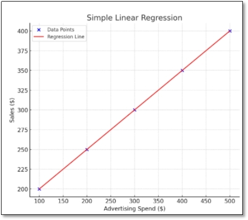
Scenario: A small retail store wants to predict monthly sales (in $) based on advertising spend (in $).

Dataset:

Month	Advertising Spend (X)	Sales (Y)
1	100	200
2	200	250
3	300	300
4	400	350
5	500	400

Step-by-Step Solution:

1. Plot data: Visualize X vs Y; the trend is roughly linear.

2. Equation form : Y= a+bX

3. Calculate slope (b):

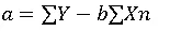
4. Calculate intercept (a):

5. Prediction: If advertising = $600, predict sales:

Y = a + b(600)

6. Interpretation: For every $1 spent on advertising, sales increase by b dollars.

2. Multiple Linear Regression – Many Factors at Play

When one factor isn’t enough to explain an outcome, we use multiple linear regression (MLR). It models the relationship between a dependent variable and two or more independent variables.

Here, each independent variable (X1, X2…Xn) has its own coefficient showing its effect on Y.

When to Use Multiple Regression

i. When multiple factors influence an outcome.

ii. To control for confounding variables.

iii. To improve prediction accuracy.

Assumptions & Multicollinearity Issues

MLR has the same assumptions as simple regression, but with an added challenge: multicollinearity, when independent variables are highly correlated with each other. This can make it difficult to assess individual variable importance. Variance Inflation Factor (VIF) is often used to detect multicollinearity.

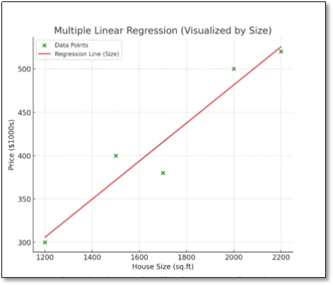
Real-Life Example

Scenario: Predict house price (in $1000s) using size (sq.ft) and number of bedrooms.

Dataset:

House	Size (X1)	Bedrooms (X2)	Price (Y)
1	1200	3	300
2	1500	4	400
3	1700	3	380
4	2000	5	500
5	2200	4	520

Step-by-Step Solution:

Equation form:   Y = a + b 1X1 + b2X2

Matrix method or software: Compute coefficients a, b1, b2a, b_1, b_2a, b1​, b2​ using regression formula.

Result (example coefficients):

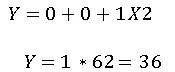
4. Prediction: For a 1800 sq.ft, 4-bedroom house:

5. Interpretation: Every extra 1 sq.ft increases price by $200 (since unit = 1000), each bedroom adds $20,000.

3. Polynomial Regression – When Life Isn’t a Straight Line

Polynomial regression is used when the relationship between variables is non-linear but still continuous. The model equation includes higher-order terms of X:

Difference from Linear Regression

While linear regression fits a straight line, polynomial regression fits a curve to better capture complex patterns.

Overfitting Risks & How to Manage Them

i. Higher-degree polynomials can perfectly fit training data but fail in real predictions.

ii. Regularization methods or cross-validation can help manage overfitting.

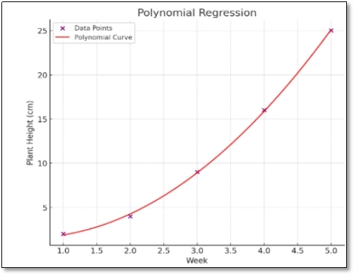
Real-Life Example

Scenario: Modeling plant growth (cm) over time (weeks), which is non-linear.

Dataset:

Week (X)	Plant Height (Y)
1	2
2	4
3	9
4	16
5	25

Step-by-Step Solution:

1. Visualize: Growth curve rises faster over time → non-linear.

2. Equation form:                 

3. Fit coefficients calculation:

Prediction: Week 6 →              

Interpretation: Plant growth accelerates quadratically; simple linear regression would underpredict later weeks.

4. Ridge and Lasso Regression (Regularized Regression)

When multiple variables exist but multicollinearity or overfitting occurs, Ridge and Lasso regression add penalties to coefficients, improving model stability and prediction accuracy.

Equation Form:

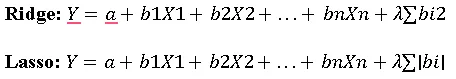
Here, λ\lambdaλ controls the penalty strength, shrinking coefficients in Ridge, and possibly setting some to zero in Lasso.

When to Use Ridge or Lasso:

i. When multicollinearity exists among independent variables.

ii. To prevent overfitting in models with many predictors.

iii. To improve prediction accuracy and simplify the model (especially Lasso).

Assumptions & Notes:

i. Same as multiple linear regression regarding linearity, homoscedasticity, and independence.

ii. Ridge keeps all variables but reduces impact of correlated ones.

iii. Lasso can remove irrelevant variables, creating a sparse, interpretable model.

Real-Life Example:

Scenario: Predict house price (in $1000s) using size (sq.ft) and number of bedrooms. Ridge or Lasso handles potential correlation if dataset is larger.

Dataset:

House	Size (X1)	Bedrooms (X2)	Price (Y)
1	1200	3	300
2	1500	4	400
3	1700	3	380
4	2000	5	500
5	2200	4	520

Step-by-Step Solution:

1. Equation Form:         

2. Compute Coefficients: Use software (Python, R, or Excel) to apply Ridge or Lasso penalty.

3. Example Result (Ridge, λ=0.1):

4. Prediction: For 1800 sq.ft, 4-bedroom house:

5. Interpretation: Ridge slightly reduces coefficients to avoid overfitting; Lasso may remove variables if irrelevant, simplifying the model.

5. Stepwise Regression – Smart Variable Selection

Stepwise regression is a technique for automatic variable selection. Instead of manually choosing predictors, the model adds or removes variables step by step based on statistical significance.

Types of Stepwise Regression

i. Forward Selection – Start with no predictors, add variables one by one until improvement stops.

ii. Backward Elimination – Start with all variables, remove the least significant ones step by step.

iii. Bidirectional Elimination – Combination of forward and backward methods.

Advantages

i. Helps in dealing with large sets of predictors.

ii. Reduces the risk of overfitting by removing unnecessary variables.

iii. Provides a cleaner, more interpretable model.

Limitations

i. May ignore theoretically important variables.

ii. Over-reliance on p-values can mislead results.

iii. Not always stable (different data samples may select different variables).

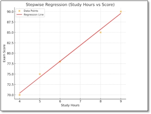
Real-Life Example

Scenario: Predict exam scores based on multiple factors: study hours (X1), sleep hours (X2), social media hours (X3), tuition classes (X4).

Dataset:

Student	Study Hours	Sleep Hours	Social Media Hours	Tuition Classes	Score
1	5	7	2	1	75
2	8	6	3	2	85
3	6	8	4	0	78
4	9	5	5	3	90
5	4	6	6	1	70

Step-by-Step Solution:

1. Start with all variables.

2. Check p-values → Remove least significant variable (e.g., Social Media Hours).

3. Re-fit model: Only Study Hours, Sleep Hours, and Tuition Classes remain.

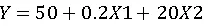
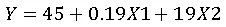
4. Final equation (example):

5. Prediction: Student with 7 study hours, 6 sleep hours, 2 tuition classes:

Interpretation: Stepwise regression identifies which factors truly matter, simplifying the model and improving predictive accuracy.

Core Assumptions You Shouldn’t Ignore

To ensure reliability, linear regression relies on these assumptions:

1. Linearity of Relationship – The dependent and independent variables must follow a linear pattern.

2. Independence of Errors – Residuals (errors) should not be correlated.

3. Homoscedasticity – Errors should have constant variance across all levels of X.

4. Normality of Residuals – Errors should be normally distributed for valid hypothesis testing.

If these assumptions are violated, results may become biased or misleading.

Measuring Model Success – Did We Predict Well?

Evaluating regression models involves checking how well predictions align with actual outcomes:

R-squared (R²): Proportion of variance explained by the model. Higher values indicate better fit.

Adjusted R-squared: Modified version of R² that penalizes for adding irrelevant predictors.

Mean Absolute Error (MAE): Average of absolute errors, easy to interpret.

Mean Squared Error (MSE): Squares errors to penalize large mistakes.

Root Mean Squared Error (RMSE): Square root of MSE, gives error in original units.

For example, if predicting monthly grocery costs, an RMSE of $200 means predictions are typically off by about $200.

Advantages of Linear Regression

1. Simplicity & Interpretability: Easy to understand, implement, and explain results to stakeholders.

2. Quick Computation: Requires less processing power and works well on small to medium datasets.

3. Insightful Relationships: Reveals how independent variables influence the dependent variable.

4. Widely Applicable: Used across business, healthcare, finance, and research for predictions and trend analysis.

5. Foundation for Advanced Models: Forms the basis for more complex machine learning techniques.

Limitations

1. Assumes Linearity: Cannot capture non-linear relationships effectively without transformation.

2. Sensitive to Outliers: Extreme values can skew results significantly.

3. Multicollinearity: Highly correlated predictors make it hard to isolate individual effects.

4. Homoscedasticity & Normality Assumptions: Violations can lead to biased or unreliable predictions.

5. Limited Flexibility: May underperform on complex or highly dynamic datasets.

Alternatives When Assumptions Are Violated

1. Ridge Regression: Reduces multicollinearity impact by adding penalty on coefficients.

2. Lasso Regression: Performs feature selection and shrinks irrelevant coefficients to zero.

3. Polynomial Regression: Captures non-linear relationships while staying interpretable.

4. Decision Trees / Random Forests: Flexible, non-parametric alternatives for complex data patterns.

5. Support Vector Regression (SVR): Handles non-linear and high-dimensional relationships efficiently.

How Simbi Labs support Businesses for Research

At Simbi Labs provides specialized services to support businesses and researchers in performing advanced linear regression analysis, enabling accurate data-driven decisions and insights.

Data Preparation & Cleaning 

Simbi Labs assists in organizing raw datasets, handling missing values, and normalizing data to ensure accurate linear regression results.

Model Selection & Customization 

Guides researchers in choosing the right type of linear regression (simple, multiple, or stepwise) based on study objectives and business needs.

Statistical Analysis & Interpretation 

Performs regression analysis, calculates coefficients, R² values, p-values, and interprets relationships between variables clearly for actionable insights.

Predictive Insights & Forecasting 

Uses regression models to predict future trends, demand, or behavior patterns, supporting strategic decision-making for businesses or research studies.

Conclusion: Why Linear Regression Still Matters

Linear regression, whether it’s basic, multiple, stepwise, or polynomial, is still a great technique to find connections in data. It helps organisations make decisions by giving them clear, predictable, and confident information. Regression is useful in many fields since it can be used to do many things, including forecasting housing values, budgeting marketing expenditures, or making product launches better.

Interesting Fact & Question for Readers

Did you know the very first use of regression dates back to the 19th century, when Sir Francis Galton studied how children’s heights “regressed” toward their parents’ average height? That’s where the term “regression” actually comes from!

Now a question for you: If you had access to customer data for your favorite brand, what would you want to predict using linear regression—pricing, demand, or customer loyalty?

Are you ready to use your data to make decisions? Get in touch with Simbi Labs right now and start your adventure with confidence. Don’t allow statistics get in the way of your study or PhD work, particularly if you’re in Pune and having trouble with your data. Let our team of specialists take care of things for you.

Book a free consultation for appointment

Email us at : grow@simbi.in

For an in-depth understanding, please refer to our book, “Academic Research Fundamentals: Research Writing and Data Analysis”. It is available as an eBook here, or you may purchase the hardcopy here .