
Multiple Linear Regression: Formula, Assumptions, Examples & SPSS Guide
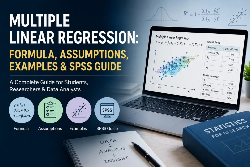
Multiple linear regression is a statistical technique used to examine the relationship between one dependent variable and two or more independent variables. It is particularly useful when an outcome is influenced by several factors and researchers need to consider those factors simultaneously.
For example, employee performance may be associated with training, work experience and job satisfaction. Rather than analysing each factor separately, multiple linear regression can estimate their relationships with performance within one model.
The method is widely applied in business, healthcare, education, finance, marketing, social sciences and academic research. It can help researchers explain patterns, identify important predictors and generate predictions. However, meaningful results depend on appropriate variable selection, data quality, assumption testing and careful interpretation.
The Fundamentals of Multiple Linear Regression
In simple terms, multiple linear regression estimates how changes in several predictor variables are associated with changes in one outcome variable.
The dependent variable is the outcome being explained or predicted. The independent variables are the predictors used to explain variation in that outcome.
For example, a researcher could study employee performance using training hours, work experience and job satisfaction as predictors.
A multiple linear regression analysis differs from correlation because correlation measures the strength and direction of association between variables, whereas regression estimates an equation that can be used to explain or predict an outcome.

Multiple Linear Regression Formula
The general multiple linear regression formula is:
Ŷ = b₀ + b₁X₁ + b₂X₂ + b₃X₃ + … + bₖXₖ
Here:
Ŷ = predicted value of the dependent variable
b₀ = intercept
b₁, b₂, b₃ … bₖ = regression coefficients
X₁, X₂, X₃ … Xₖ = independent variables
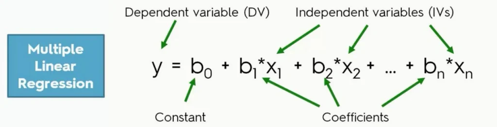
The intercept represents the predicted outcome when all predictors equal zero. Each regression coefficient indicates the expected change in the dependent variable associated with a one-unit increase in that predictor, while the other predictors remain constant.
For example, if the coefficient for training hours is 2.5, the model estimates a 2.5-unit increase in employee performance for each additional training hour, after accounting for the other predictors.
The coefficients are commonly estimated using the least-squares approach, which minimises the squared differences between observed and predicted values.
The Multiple Linear Regression Analysis Process
A reliable analysis generally follows these stages:
1. Define the research question: Establish exactly what outcome you want to explain or predict.
2. Identify variables: Select one dependent variable and relevant independent variables.
3. Prepare the data: Check coding, missing values, measurement errors and unusual observations.
4. Check assumptions: Examine linearity, independence, homoscedasticity, residual normality, multicollinearity and influential observations.
5. Run the model: Use statistical software such as SPSS to estimate the regression equation.
6. Evaluate model fit: Examine R², adjusted R² and the overall F-test.
7. Interpret coefficients: Consider B, Beta, standard errors, t-values and p-values.
8. Report findings: Explain statistical results alongside their practical and research significance.
Using Multiple Linear Regression in Research and Data Analysis
Multiple linear regression is appropriate when the dependent variable is quantitative and the research question involves several predictors.
For example, businesses can predict sales using advertising expenditure, product price and market size. Researchers can examine employee performance using experience, training and education. Healthcare studies may investigate relationships between several predictors and a continuous patient outcome, while education researchers may study academic performance using attendance, study time and prior achievement.
It should not automatically be used simply because several variables are available. A different method may be more appropriate for a categorical outcome, strongly nonlinear relationships, repeated measurements or non-independent observations. For example, IBM recommends logistic regression for dichotomous dependent variables and repeated-measures procedures when observations are not independent.
Assumptions of Multiple Linear Regression
- Linearity: The relationship between the outcome and predictors should be adequately represented by a linear model. Residual plots and scatterplots can help identify curves or systematic patterns suggesting that a linear model may not be appropriate.
- Independence of Observations: Observations should be independent of one another. Repeated measurements from the same individual or clustered observations, such as students within schools, may violate this assumption and require a different analytical approach.
- Homoscedasticity: The variance of the residuals should remain reasonably constant across predicted values. A residual-versus-predicted plot can help identify unequal variance, often visible as a funnel-shaped pattern.
- Normality of Residuals: Residuals should be approximately normally distributed for conventional statistical inference. Researchers can examine histograms and normal probability or Q-Q plots. Importantly, this assumption concerns the residuals, not necessarily every raw variable.
- Absence of Multicollinearity: Predictors should not be excessively correlated with one another. Strong multicollinearity can make coefficients unstable and increase standard errors. VIF and Tolerance statistics are commonly used as diagnostics.
- Absence of Significant Outliers: Unusual observations can have a disproportionate effect on the regression equation. Researchers should examine residuals, leverage and influence measures rather than automatically deleting observations.
How to Perform Multiple Linear Regression in SPSS
Step 1: Prepare Your Dataset
Check that the dependent and independent variables are correctly coded and that missing or invalid observations have been reviewed.
Step 2: Open Linear Regression
In SPSS,
Go to the Analyze menu, select Regression, and then choose Linear.
Step 3: Select the Dependent Variable
Move the continuous outcome variable into the Dependent box.
Step 4: Add Independent Variables
Move the selected predictors into the Independent(s) box.
Step 5: Select Statistics and Diagnostics
Request relevant model-fit statistics, confidence intervals and collinearity diagnostics. Residual plots can also be requested to evaluate model assumptions.
Step 6: Run the Analysis
Select OK to generate the regression output.
Step 7: Examine the SPSS Output
The main tables include the Model Summary, ANOVA and Coefficients tables. SPSS also provides diagnostic statistics and plots that can support assumption checking.
Multiple Linear Regression Example
Consider a company attempting to understand its monthly sales. Suppose analysts collect information about:
A. Advertising expenditure
B. Website visits
C. Number of sales representatives
D. Monthly sales revenue
Here, monthly sales revenue is the dependent variable, while advertising expenditure, website visits and sales representatives are independent variables.
Suppose the resulting model is:
Sales = 20,000 + 2.5(Advertising) + 0.8(Website Visits) + 1,200(Sales Representatives)
The coefficients provide information about the estimated relationship between each predictor and sales. For example, the coefficient for advertising indicates the expected change in sales associated with a one-unit increase in advertising expenditure, assuming website visits and the number of sales representatives remain unchanged.
How to Interpret Multiple Linear Regression Results
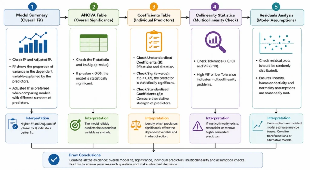
a.Model Summary: The Model Summary includes R, R Square, Adjusted R Square and Standard Error of the Estimate.
R² represents the proportion of variation in the dependent variable explained by the predictors. For example, R² = 0.60 means that the model explains 60% of the variation in the outcome within the analysed sample.Adjusted R² accounts for the number of predictors and sample size. It is particularly useful when comparing models containing different numbers of predictors.
b. ANOVA Table: The ANOVA table reports the F-statistic and significance value. The overall F-test evaluates whether the regression model, considered as a whole, provides evidence of an association between the predictors and the dependent variable.
c. Coefficients Table: The Coefficients table contains B, Standard Error, Beta, t and Sig. B represents the unstandardized coefficient and is interpreted in the original units of the variable. Beta is the standardized coefficient and can assist in comparing predictors measured on different scales.
The t-value and p-value are used to assess individual coefficients.
d. Collinearity Statistics: Tolerance and VIF help identify multicollinearity. High multicollinearity can make coefficient estimates less stable and complicate regression results interpretation. SPSS includes VIF and Tolerance among its available regression statistics.
Multiple Linear Regression vs Simple Linear Regression
| Feature | Simple Linear Regression | Multiple Linear Regression |
| Dependent variable | 1 | 1 |
| Independent variables | 1 | 2 or more |
| Purpose | Prediction/explanation | Prediction/explanation using multiple predictors |
| Example | Sales → Advertising | Sales → Advertising + Price + Market Size |
Advantages and Limitations of Multiple Linear Regression
Advantages
Multiple linear regression can analyse several predictors simultaneously, estimate their individual relationships with an outcome and provide a framework for prediction. It can also account statistically for other measured predictors when examining a particular variable.
Limitations
Results can be affected by multicollinearity, outliers, assumption violations, poor data quality and inappropriate model specification. Adding more predictors does not automatically produce a better model. Most importantly, statistical association does not automatically establish causation.
Common Mistakes in Multiple Linear Regression
Researchers should avoid several common problems:
1. Ignoring regression assumptions.
2. Including highly correlated predictors without assessing multicollinearity.
3. Treating a significant p-value as proof of causation.
4. Reporting R² without considering adjusted R² and model diagnostics.
5. Including too many predictors relative to the available sample.
6. Ignoring influential observations.
7. Focusing only on statistical significance while overlooking the size and practical meaning of coefficients.
Applications of Multiple Linear Regression
Multiple linear regression has broad applications. In healthcare, it can examine factors associated with continuous health outcomes. In business, it can support sales and revenue modelling. Marketing researchers can examine factors associated with customer behaviour, while education researchers can study academic performance. In finance, regression can investigate relationships involving financial outcomes, and in social sciences, it can examine behavioural and demographic predictors.
Multiple Linear Regression Analysis Services
A sound regression analysis requires appropriate model selection, data preparation, assumption testing and interpretation—not simply running the analysis in software.
Simbi Labs provides statistical analysis support for researchers, PhD scholars, businesses and organisations. Support can include data cleaning, variable selection, regression model development, assumption testing, SPSS regression analysis, output interpretation and statistical reporting.
For researchers seeking multiple linear regression analysis services or SPSS regression analysis services, professional statistical support can help ensure that the selected methodology and interpretation are appropriate for the research objectives.
Book a free consultation for appointment
Email us at : grow@simbi.in
Frequently Asked Questions About Multiple Linear Regression
What is multiple linear regression?
It is a statistical method for examining one dependent variable using two or more independent variables.
What is the difference between simple and multiple linear regression?
Simple regression uses one predictor, whereas multiple regression uses two or more predictors.
What is the formula for multiple linear regression?
The general equation is Ŷ = b₀ + b₁X₁ + b₂X₂ + … + bₖXₖ.
What are the assumptions of multiple linear regression?
Key assumptions include linearity, independence, homoscedasticity, appropriate residual behaviour, absence of problematic multicollinearity and assessment of influential observations.
When should multiple linear regression be used?
It is generally used when a quantitative outcome is being examined in relation to two or more predictors.
How do you interpret R-squared in multiple regression?
R² indicates the proportion of variation in the dependent variable explained by the predictors in the fitted model.
What is adjusted R-squared?
Adjusted R² accounts for the number of predictors and sample size and is useful when comparing models with different numbers of predictors.
What is multicollinearity in multiple linear regression?
It occurs when predictors are strongly related to each other, potentially making individual coefficients unstable.
How do you interpret regression coefficients?
A coefficient indicates the expected change in the dependent variable associated with a one-unit change in a predictor while holding the other predictors constant.
What does a significant p-value mean in multiple regression?
It indicates evidence against the null hypothesis that the tested coefficient equals zero, assuming the model and statistical conditions are appropriate.
Can multiple linear regression be used for prediction?
Yes. It can generate predicted values from multiple predictors, although prediction quality depends on data quality, model specification and generalisability.