
Power Analysis for Proportions in SPSS

Introduction
Statistical power analysis is a crucial step in research planning. It helps you determine how large a sample you need to detect an effect of interest, or conversely, what the probability is of detecting that effect given your existing data. Conducting power analysis before a study can save time, resources, and prevent inconclusive results.
While power analysis for means deals with continuous data (e.g., height, weight, scores), power analysis for proportions is focused on binary outcomes — situations where there are only two possible categories such as:
Pass / Fail
Yes / No
Improved / Not Improved
Success / Failure
In many real-world cases — such as medical trials, education research, quality control, or survey analysis — outcomes are recorded as proportions. In such cases, using the correct test and performing an accurate power analysis is essential to avoid Type II errors (failing to detect a real effect).
This blog will guide you through power analysis for proportions in SPSS, starting with the One-Sample Binomial Test, followed by Related-Sample Binomial Test and Independent-Sample Binomial Test in subsequent sections.
Read Also : How to Perform Power Analysis for Means in SPSS: Step-by-Step Guide with Examples
A. What is One-Sample Binomial Test – Power Analysis in SPSS?
Purpose of the Test
The One-Sample Binomial Test is used when you want to test whether the proportion of “successes” in your sample is significantly different from a known or hypothesized population proportion.
Example:
A teacher wants to evaluate whether her class’s pass rate on a final exam is different from the historical pass rate of 50%.
She collects results from 50 students and records whether each passed or failed.
What is the goal of the Analysis?
Power Analysis Goal: Assess whether the current sample size is large enough to detect a small difference (such as 0.52 vs. 0.50), and if not, estimate the required sample size for 80% power.
Hypothetical Data
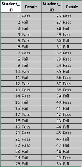
Summary Table:
| Result | Count | Proportion |
| Pass | 26 | 0.52 |
| Fail | 24 | 0.48 |
| Total | 50 | 1.00 |
Hypothesis:
Null Hypothesis (H₀): p = 0.50
Alternative Hypothesis (H₁): p ≠ 0.50
Significance Level: α = 0.05
What are Steps in SPSS?
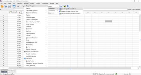
Step 1 – Open the Power Analysis Window
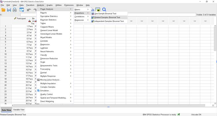
In SPSS, go to:
Analyze > Power Analysis > Proportion > One-Sample Binomial Test
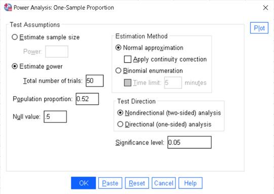
Step 2 – Enter Values for Achieved Power
Since we want to calculate the achieved power for our existing dataset:
i. Select: Estimate power
ii. Total number of trials: 50
iii. Population proportion: 0.52 (observed proportion from the dataset)
iv. Null value: 0.5
v. Estimation Method: Keep Normal approximation (you can also try Binomial enumeration for exact results)
vi. Test Direction: Nondirectional (two-sided)
vii Significance level: 0.05
Step 3 – Run the Analysis
Click OK.
How to write interpretation of for a One-Sample Binomial Test in SPSS?
The achieved statistical power for the one-sample binomial test, based on a two-sided normal approximation, is 0.059 (5.9%). This means that with a sample size of 50 and a true proportion of 0.52 compared to the null hypothesis proportion of 0.50 at a 5% significance level, there is only a 5.9% chance of correctly rejecting the null hypothesis if the alternative hypothesis is true. This is far below the commonly recommended 80% power, indicating the study is severely underpowered to detect such a small difference.
B. What is Related Samples Binomial Test – Power Analysis in SPSS?
SPSS
Purpose of Test:
The Related-Samples Binomial Test is used when you have paired binary outcomes (e.g., before/after results for the same subjects, or two related conditions) and you want to know if the probability of success is the same in both situations.
In SPSS, the Power Analysis option for the Related-Samples Binomial Test allows you to:
i. Calculate the achieved power for your paired data.
ii. Example:
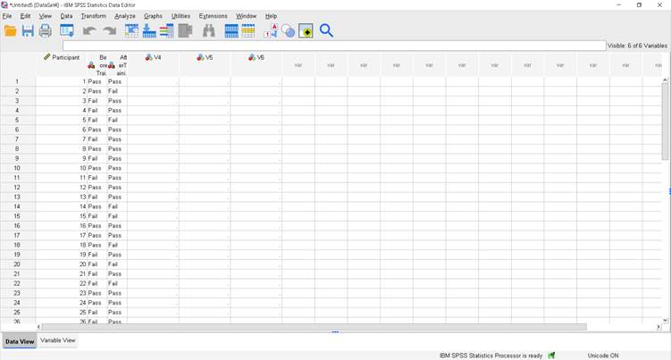
A researcher wants to test whether a training program improves employees’ certification pass rates compared to before the training.
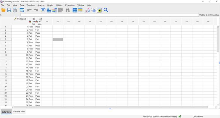
They record the pass/fail results of the same 40 employees before and after the program.
What is Goal of Power Analysis?
Determine whether the current sample size (n = 40 paired observations) is sufficient to detect the observed change in pass rates between the two related conditions, and if not, estimate the sample size needed to achieve 80% power.
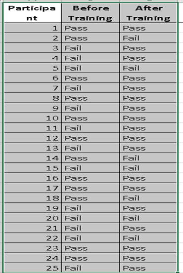
Summarizing Results
Pass → Pass: 12
Pass → Fail: 5
Fail → Pass: 14
Fail → Fail: 9
Total participants: 40
Discordant pairs = Pass→Fail (5) + Fail→Pass (14) = 19
Calculating Observed Proportion
We define “success” as improvement (Fail → Pass):
Observed proportion=1419≈0.737
Hypotheses
H₀: Probability of improvement = 0.5
H₁: Probability of improvement ≠ 0.5
What are steps in SPSS?
Step 1 – Open the Power Analysis Window
In SPSS, go to:
Analyze > Power Analysis > Proportion > Related-Sample Binomial Test
Step 2 – Enter Values for Achieved Power
Since we want to calculate the achieved power for our existing dataset:
i. Select: Estimate power
ii. Total number of trials: 40
iii. Population proportion1: 0.35 (before the treatment dataset)
iv. Population proportion2: 0.65(after the treatment)
v. Estimation Method: Keep Normal approximation (you can also try Binomial enumeration for exact results)
vi. Test Direction: Nondirectional (two-sided)
vii. Significance level: 0.05
Step 3 – Run the Analysis
Click OK.
How to write interpretation of Related Samples Binomial Test – Power Analysis in SPSS?
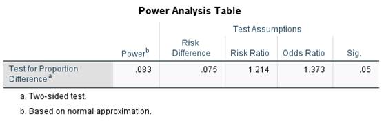
The power value (0.083) indicates only an 8.3% chance of detecting the observed difference between the two proportions at the 5% significance level, which is far below the commonly desired 80%.
The observed risk difference is 0.075, meaning the second group’s success rate is 7.5 percentage points higher than the first.
The risk ratio (1.214) shows the probability of success is about 21% higher in the second group, while the odds ratio (1.373) indicates the odds are roughly 37% higher.
Given the low power, the sample size is insufficient to reliably detect this difference, and results should be interpreted with caution.
Read Also : Power Analysis for Pearson Correlation in SPSS
C. What is Independent-Sample Proportions (Binomial Test) in Power Analysis in SPSS?
The Independent-Samples Binomial Test is used when you want to compare proportions between two different, unrelated groups. It helps you determine the required sample size or the statistical power needed for detecting a difference in proportions between these groups.
In SPSS, this is accessed via:
Analyze > Power Analysis > Proportion > Independent-Samples Binomial Test
Purpose of Power Analysis
Power analysis answers two important research design questions:
1. How many samples are needed to detect a difference between groups with a certain probability (power)?
2. How much power you have given a certain sample size.
Example:
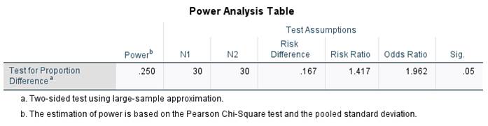
With only 30 households per village, the study has just 25% power to detect a 16.7% difference in livestock loss rates between the two villages, making it likely that a true effect could be missed.
The odds of loss are nearly twice as high in Village A compared to Village B, but the low power limits confidence in detecting this difference.
Hypothetical Dataset
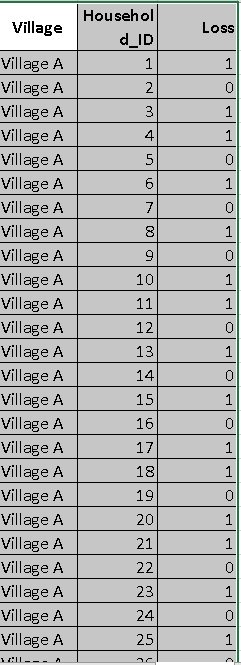
Summary of Data table:
| Village | Loss Reported (1) | No Loss (0) | Total | Proportion |
| Village A | 17 | 13 | 30 | 0.5667 |
| Village B | 12 | 18 | 30 | 0.4000 |
Hypotheses
Null hypothesis (H₀):
p1=p2
The proportion of households reporting livestock loss is the same in both villages.
Alternative hypothesis (H₁):
p1≠p2
The proportion of households reporting livestock loss is different between the two villages.
What are steps in SPSS?
Step 1 – Open the Power Analysis Window
In SPSS, go to:
Analyze > Power Analysis > Proportion > Independent-Sample Binomial Test

Step-2
How to Fill up SPSS Dialogue Box?

Top-left: Estimate power
We want SPSS to compute the power for the sample sizes you already have.
Total number of trials for group 1: 30
Total number of trials for group 2: 30
Explanation: you provided 30 households in Village A and 30 in Village B.
Proportion parameters for group 1: 0.5667
How calculated: Village A had 17 households reporting loss out of 30.
Prop1=17/30=0.566666 round to 0.5667.
Proportion parameters for group 2: 0.4000
How calculated: Village B had 12 households reporting loss out of 30.
Prop2=12/30=0.4 Significance level: 0.05
Standard α = 0.05 for a two-sided test.
Test Method: Chi-squared test (leave “Standard deviation is pooled” checked)
Explanation: this is the usual large-sample method for comparing two independent proportions (equivalent to a two-sample z test). “Pooled” means the standard error used in the test is computed from the pooled proportion under H₀.
Apply continuity correction: optional (I usually leave unchecked for power estimation — it makes the test slightly more conservative and reduces power).
Estimation Method: Normal approximation
With n = 30 per group normal approximation is acceptable. (If you want exact results you could choose Binomial enumeration, which is slower but exact.)
Test Direction: Nondirectional (two-sided)
Because we’re testing p1≠p2
Step 3 – Run the Analysis
Click OK.
How to write interpretation of Related samples binomial test in Power Analysis?
This table shows that with 30 participants in each group (N1 = 30, N2 = 30), the study has a statistical power of 0.250 (25%), which is relatively low for detecting the effect.
The risk difference between groups is 0.167, indicating a 16.7% higher proportion in one group compared to the other.
The risk ratio is 1.417, meaning the event is 41.7% more likely in one group, while the odds ratio of 1.962 suggests nearly double the odds.
The significance level is set at 0.05, and results are based on a two-sided Pearson Chi-Square test using pooled standard deviation.
For an in-depth understanding, please refer to our book, “Academic Research Fundamentals: Research Writing and Data Analysis”. It is available as an eBook here, or you may purchase the hardcopy here .