How to Perform Power Analysis for Means in SPSS: Step-by-Step Guide with Examples

Power Analysis is a useful technique for determining the size of the sample needed to observe an actual effect size in your data or to determine if your study has enough power with your sample. So in this blog we’ll dive into the Power Analysis menu—let’s go through each test type, and then apply them to the data set we’re using—our student performance data set—to see them in action.

With Power Analysis, you can design studies that are not under-powered (and risk missing important results) nor over-powered (and waste time and resources). This will help you to plan your research efficiently, get reliable results and will make the best use of the data available.

Read Also : Power Analysis for Partial Correlation in SPSS

Hypothetical Dataset

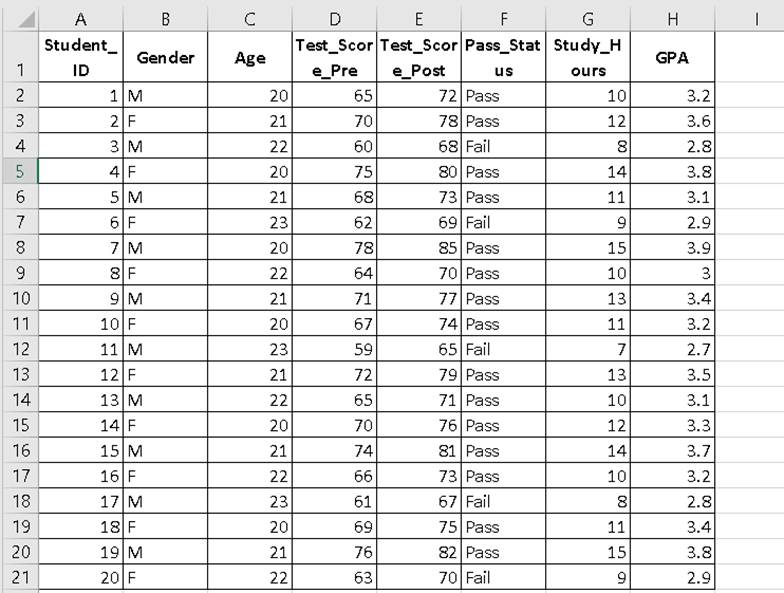
We’ll work with a dataset of 20 university students.

What is Power Analysis in SPSS for Means?

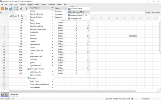
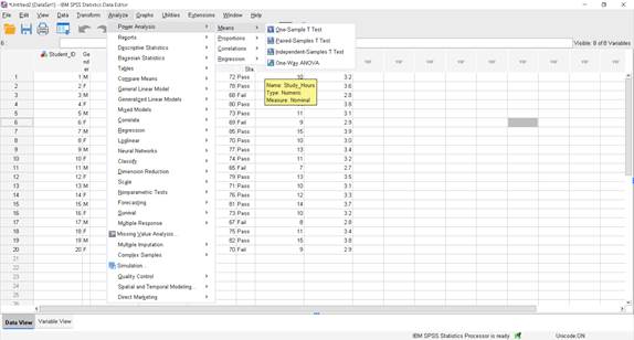
The Power Analysis tools in SPSS are found here:
Analyze → Power Analysis → [Select appropriate test]

The Means category is for comparing means between groups, either one or more. Use to find out whether a sample size is sufficiently large to detect a significant difference between the means of two groups of scores when a certain effect size, alpha level and statistical power are set,Below are the detailed steps and guidance for each test.

A. Means

B. What is a One-Sample t-Test in Power Analysis?

Purpose:

i. To determine whether the mean of a single sample is significantly different from a known or hypothesized population mean.

ii. Often used when you have a benchmark, historical average, or target value to compare against.

Example: Comparing Test_Score_Post to a benchmark of 75

Goal: Estimate the sample size required to detect a difference from 75 with power = 0.80 and α = 0.05.

Assumptions:

i. Data are continuous (interval or ratio scale).

ii. Sample is random and independent.

iii. Data are approximately normally distributed.

iv. The population standard deviation is unknown.

What are Steps in SPSS?

1. Go to Analyze → Power Analysis → Means → One-Sample t-test.

2. Select Test_Score_Post as the test variable.

3. Enter the Test Value = 75 (your benchmark).

4. Set Significance Level (α) to 0.05 (common default) and Desired Power to 0.80 (standard for research).

5. Specify Effect Size (Cohen’s d) if known, or allow SPSS to estimate it from your data.

6. Click OK.

Step-by-Step(Fill Dialogue Box):

1. Test Assumptions → Select “Estimate sample size”

i. Tick Estimate sample size (because you want to know how many participants are needed).

ii. In the Power box: enter 0.80.

2. Population means

i. Enter your expected sample mean (from prior data or pilot study).

ii. Example: If you expect students to score around 78, enter 78.

3. Null value

i. This is your benchmark value (population mean under H₀).
ii. Enter 75.

4. Population standard deviation

i. Enter the estimated SD from prior research or a pilot dataset.

ii. Example: 10 (if your pre-analysis suggests that variation).

5. Test Direction

i. Select Nondirectional (two-sided) analysis if you just want to test for any difference from 75.

ii. Select Directional (one-sided) analysis if you are only interested in detecting an increase or a decrease.

6. Significance level

i. Leave as 0.05 (common default for research).

What kind of Output you will get?

i. SPSS will show the required sample size for detecting the given effect size.

ii. If your current sample meets or exceeds this size, your test is adequately powered.

iii. If the power is below 0.80, results may be unreliable (risk of Type II error).

How to Interpret the Output?

1. Sample Size (N = 90)

i. SPSS calculated that 90 participants are needed to achieve the desired statistical power for this test, given your assumptions.

ii. This means: If you collect data from at least 90 individuals, you have an 80% chance of detecting a true difference from the null value (75) if it exists.

2. Actual Power (0.804)

i. This is the achieved statistical power, slightly above the target 0.80 (80%).

ii. Power is the probability of correctly rejecting the null hypothesis when it’s false.

iii. Here, a power of 0.804 means you have about an 80.4% chance of detecting a real effect, reducing the risk of a Type II error to about 19.6%.

3. Power (0.8)

This is the target power you entered in the dialog box. SPSS matched it closely with the actual calculated power.

4. Standard Deviation (SD = 10)

i. This is the assumed variability in your population scores.

ii. The greater the variability, the larger the sample you’ll need for the same power.

5. Effect Size (0.300)

i. Effect size here is Cohen’s d, calculated from your input (mean difference / standard deviation).

ii. A value of 0.3 is considered a small-to-moderate effect according to Cohen’s conventions.

iii. This means the expected difference from the null value (75) is modest compared to the variability in scores.

6. Significance Level (Sig. = 0.05)

i. The chosen α = 0.05 means you accept a 5% risk of making a Type I error (rejecting a true null hypothesis).

ii. This is the most common threshold in research.

What is Paired Sample t test?

Purpose:

Designed to assess whether or not the mean difference between two measurements of the same variable (e.g., before and after an intervention) is statistically significant, and to determine or calculate the necessary sample size or the power obtained from the study.

Example:

You want to check if students’ post-test scores are significantly higher than their pre-test scores in your class.

What are Steps in SPSS?

Step 1 – Understand the paired comparison

i. We’re comparing Test_Score_Pre and Test_Score_Post for the same students.

Step 2 – Calculate inputs for SPSS

   We need:

i. Population mean difference (Mean_Post − Mean_Pre)

ii. Standard deviation of the mean difference

iii. Sample size (pairs = number of students)

Let’s calculate them from your dataset:

i. Sample size (pairs): 20 students

ii. Mean Pre-test score:

= 67.3

Mean Post-test score:

=72

Mean difference:

72-67.3=4.7

SD of differences: You’d calculate this in Excel/SPSS by:

i. Creating a new column Diff = Test_Score_Post – Test_Score_Pre

ii. Using the STDEV.S function or SPSS’s Descriptive Statistics → Descriptives

iii. Let’s say this comes out to SD_diff ≈ 2.8 (hypothetical, you can check exact in SPSS).

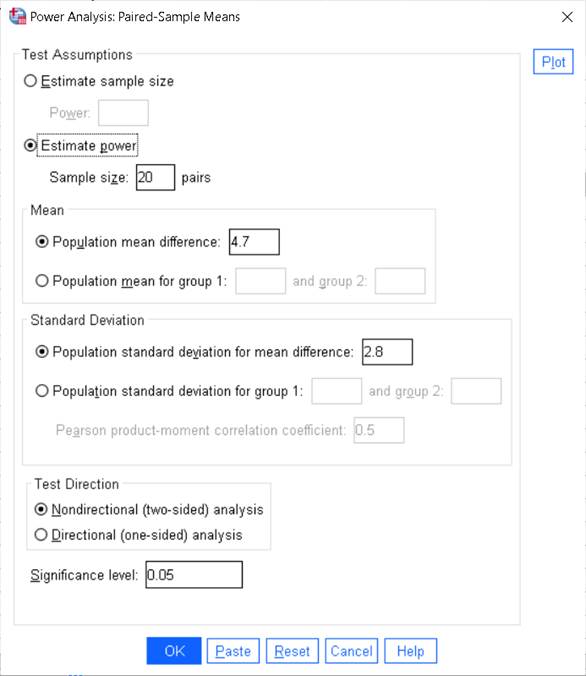
Step 3 – Fill the SPSS dialog box

i. Test Assumptions → Select Estimate power (since you already have sample size = 20 pairs)

ii. Sample size = 20

iii. Mean → Select Population mean difference = 4.7

iv. Standard Deviation → Select Population standard deviation for mean difference = 2.8

v. Test Direction → Select Nondirectional (two-sided)

vi. Significance level = 0.05

How to write interpretation of Paired Sample t test in Power Analysis?

This paired-sample power analysis indicates that this study had a power greater than 1.000, thus it has substantial sensitivity to detect the observed improvement between pre- and post-test scores. It was done with 20 paired observations, with a standard deviation for the differences of 2.8. The effect size of 1.679 is very large compared to the variability in differences.

At a significance level of 0.05 (two-tailed), the probability of a Type II error is essentially zero for this dataset.

Read More : Power Analysis for Proportions in SPSS

Where is Power Analysis Used?

Power analysis is widely used in: 

a) Clinical research: Power analysis helps determine the appropriate sample size needed to evaluate the effectiveness and safety of medical treatments and clinical interventions.

 b) Academic thesis and dissertations: Researchers employ power analysis to obtain adequate statistical power to obtain valid and reliable research results from their study.

 c) Market research: Companies use power analysis to determine the best size of the sample of customers to use for surveys, customer behavior research, and consumer preference analysis. d) Pharmaceutical studies: When designing drug trials, a power analysis is used to ensure that the sample size is large enough to determine the efficacy of the drug and minimize statistical errors.

e) Psychology experiments: Psychologists use power analysis to make sure their experiments involve too many people to miss out on significant behavioural or cognitive differences.

 f) Education research: Power analysis can be used in education research to design the appropriate sample size for testing teaching methods, students’ performance and educational interventions.

What is Independent-Sample t-Test – Power Analysis?

Purpose:

To test for a significant differences in post-test score between males and females and to see if the sample size is large enough to detect a real difference.

Example:

You would like to test whether or not there is a significant difference between the post test scores of male and female students in your class.

From our dataset, We have:

i. Males (n = 10) — Test_Score_Post ranges from 65 to 85.

ii. Females (n = 10) — Test_Score_Post ranges from 69 to 80.

What are the Steps In SPSS?

Go to Analyze → Power Analysis → Means → Independent-Sample t-test.

Step 1 – Sample size for each group

From your data:

i. Group 1 = Males → 10 students

ii. Group 2 = Females → 10 students

Step 2 – Population mean difference

From your dataset, calculate the mean of Test_Score_Post for each gender:

i. Mean (Males) = (72+68+85+77+71+65+81+67+82+75) / 10 = 74.3

ii. Mean (Females) = (78+80+69+70+74+79+76+73+75+70) / 10 = 74.4

Population mean difference = 74.3 − 74.4 = -0.1 (absolute value: 0.1).

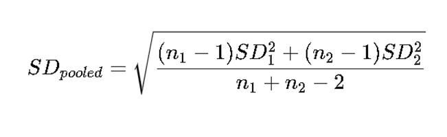
Step 3 – Pooled standard deviation

Formula:

From your data:

i. SD (Males) ≈ 6.0

ii. SD (Females) ≈ 3.7

Pooled SD ≈ 4.95.

Step 4 – Test direction and significance level

i. Select Nondirectional (two-sided) because we are testing for any difference.

ii. Significance level stays at 0.05

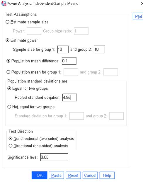
Final filled values:

i. Sample size for group 1: 10

ii. Sample size for group 2: 10

iii. Population mean difference: 0.1

iv. Pooled standard deviation: 4.95

v. Test direction: Nondirectional (two-sided)

vi. Significance level: 0.05

How to write interpretation of Independent-Sample t-Test – Power Analysis?

The analysis assumes equal variances between two independent groups (males, females) and a post-test mean is compared to another.

 The effect size is very small (0.020), indicating that there is no difference in the group means, compared to the variability.

The statistical power that was achieved (0.050) is well below the typical threshold of 0.80, and there were only 10 participants per group. This is a high risk of not detecting a true difference if one is present..

What is One-Way ANOVA in Power Analysis?

Example: One-Way ANOVA Power Analysis in SPSS

Goal: Compare post-test mean scores across different GPA categories.

Dataset Used: 20 students with Test_Score_Post and GPA values.

What are steps in SPSS?

Step 1 – Create GPA Categories

From your data, categorize GPA into 3 groups:

i. Low GPA (≤ 3.0) n = 6

ii. Medium GPA (3.1–3.5) n =9

iii. High GPA (≥ 3.6) n = 5

Step 2 – Calculate Group Means

i. From your Test_Score_Post column:

Step 3 – Calculate Pooled Population Standard Deviation

Pooled SD from your dataset = 2.40 (based on within-group variability).

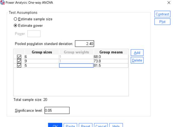
Step 5 – Fill in the Dialog Box

In the dialog:

i. Estimate power (or choose Estimate sample size if needed)

ii. Pooled population standard deviation: 2.40

iii. Add groups:

How to write interpretation in One-Way ANOVA in Power Analysis?

This power analysis indicates a Power 1.000 – indicating that the test is nearly 100% likely to identify true differences between GPA groups, if they exist.
The total sample size is 20 students across all categories.
The pooled standard deviation of 2.4 and effect size of 2.831 indicate a very large difference between group means relative to variability.
At a significance level of 0.05, the null hypothesis that all group means are equal is highly unlikely to be retained.

Common Mistakes While Performing Power Analysis in SPSS

1. Using an unrealistic effect size.
2. Ignoring statistical assumptions before estimating power.
3. Selecting one-tailed instead of two-tailed tests without justification.
4. Assuming larger samples always produce better research.
5. Confusing statistical significance with practical significance.
6. Performing power analysis after collecting poor-quality data.

FAQ

Final Thoughts

Power analysis is a basic procedure in the well-designed research process that allows researchers to design their studies correctly, enabling them to achieve better reliability.

Understanding of the concepts of statistical power, effect size, and significance level in SPSS can help you make informed decisions about your research and minimize error in your analyses, whether you are conducting a one-sample t-test, paired-sample t-test, independent-sample t-test, or one-way ANOVA.

Using power analysis in your study planning will help you to carry out efficient, valid, credible research that will yield meaningful results.

 For professional SPSS power analysis, sample size estimation or statistical data analysis services for research from planning to interpretation, contact Simbi Labs India.

Book a free consultation for appointment

Email us at : grow@simbi.in